Using lme4, I show why random slopes is often needed in biomedical research and experiments
Author
Daniel S. Mazhari-Jensen
Published
July 23, 2025
Multi-level models and why random slopes matter
How two memes helped me learn something about mixed-effect models
About six months ago, I came across these two memes:
Meme 1
Meme 2
At first, I was genuinely puzzled. What exactly is the connection between adding a random intercept in a regression model and inflating Type I error when you don’t include a random slope?
If you, like I did, got intrigued by these meme’s nuggets of information, consider reading along.
My goal here is to unpack what’s going on in a way that’s accessible, honest, and hopefully a little enjoyable. I’m not writing a textbook chapter; this is more of a personal explanation of a concept I found tricky and later came to appreciate.
⚠️ Note: I assume you have a basic understanding of regression models and null-significance-hypothesis-tests. What follows is not a deep statistical dive, but it should give you just enough to understand the meme, avoid a common pitfall, and get curious about mixed-effects models. The material is based on:
Gelman, A., & Hill, J. (2007). Data analysis using regression and multilevel/hierarchical models. Cambridge university press. **A comprehensive book on the topic of *multilevel models**
Barr, D. J., Levy, R., Scheepers, C., & Tily, H. J. (2013). Random effects structure for confirmatory hypothesis testing: Keep it maximal. Journal of memory and language, 68(3), 255-278. A simulation study showing the type-1 error problem of random intercept only models
Gelman, A. (2005). Analysis of variance—why it is more important than ever.
How we’ll approach it:
We’ll focus on why random slopes are crucial in many types of data—especially in biometric or health science research, where repeated measures designs are common. We’ll use a small simulation in R to illustrate the key concepts, relying on vanillalme4 and some tidyverse-styled data wrangling.
The data set we’ll use to demonstrate this comes from a simple simulation that mimics a common experimental design: repeated measures of a response variable (here: reaction time) across multiple sessions per participant.
Imagine we are testing whether people improve (get faster) with repeated practice. This is a typical setup in cognitive psychology. Often, researchers want to know: is there a significant learning effect over time?
We might want to investigate whether a test we’re performing has an undesirable shift across multiple repeated measures (stability of test instrument) in order to validate it and show it’s feasibility as a repeated measure for a clinical trial, for example for a medical assessment for driving skills under the influence of a given drug.
But here’s the issue (SPOILER ALLERT!): if you don’t model the data closely, you might get fundamentally different results!
Let’s dive in and see why.
Simulating our data set:
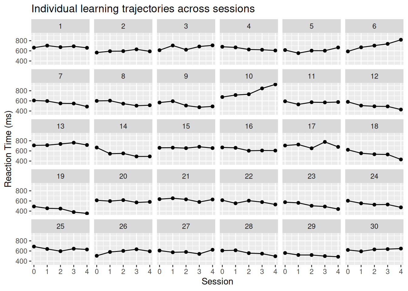
We simulate a data set where each subject completes five sessions of a task. There’s a general trend toward faster responses over time, but with subject-specific differences in both starting reaction time and learning rate.
Code
set.seed(314)# Parametersn_subjects <-30n_sessions <-5# Fixed effect of session: general learning effectbeta_0 <-600# Average baseline RT in msbeta_1 <--10# Average decrease in RT per session# Random effects: standard deviationssd_intercept <-50# SD of baseline RTs across subjectssd_slope <-25# SD of learning rates (slopes)rho <-0.2# Correlation between intercepts and slopes# Within-subject residual errorsigma_error <-30# Construct subject-level random effects (correlated)subject_re <- MASS::mvrnorm(n = n_subjects,mu =c(0, 0),Sigma =matrix(c(sd_intercept^2, rho*sd_intercept*sd_slope, rho*sd_intercept*sd_slope, sd_slope^2), 2)) |>as.data.frame() |>setNames(c("intercept_re", "slope_re")) |> dplyr::mutate(subject =factor(1:n_subjects))# Create session vector repeated for each subjectsession <-rep(0:(n_sessions -1), times = n_subjects)# Repeat subject IDs for each sessionsubject <-rep(subject_re$subject, each = n_sessions)# Join the random effectssim_data <- tibble::tibble(subject = subject, session = session) |> dplyr::left_join(subject_re, by ="subject") |> dplyr::mutate(reaction_time = beta_0 + intercept_re + (beta_1 + slope_re) * session +rnorm(dplyr::n(), mean =0, sd = sigma_error) )
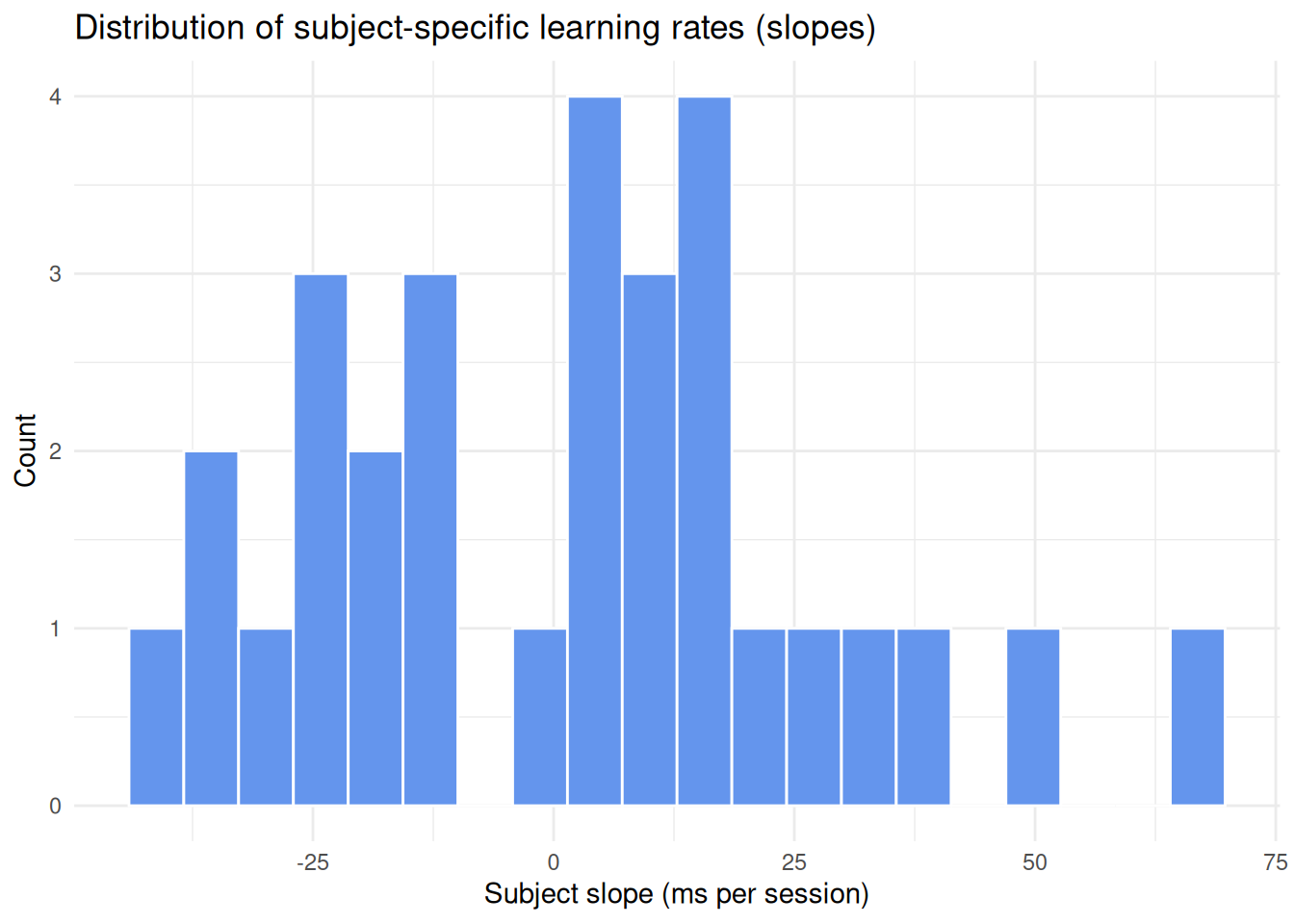
Here’s the distribution of slopes (ie. learning rate variability):
Code
subject_re |>ggplot(aes(x = slope_re)) +geom_histogram(bins =20, fill ="#6495ED", color ="white") +labs(title ="Distribution of subject-specific learning rates (slopes)",x ="Subject slope (ms per session)", y ="Count") +theme_minimal()
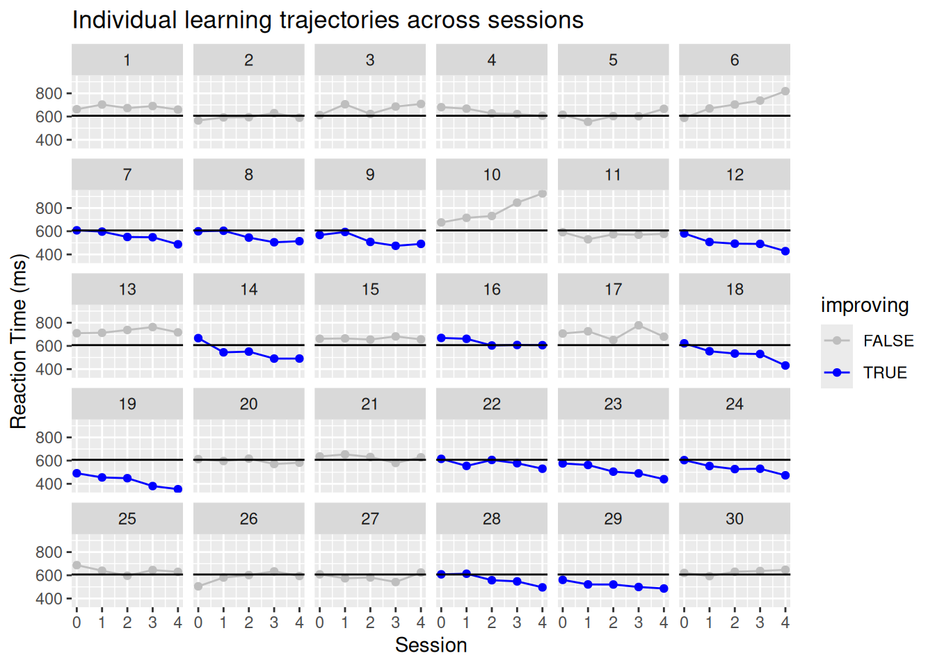
sim_data |>ggplot(aes(y=reaction_time, x=session)) +facet_wrap(~ subject, ncol=6) +geom_point() +geom_line() +scale_x_continuous(limits=c(0, 4),breaks=c(0:4)) +labs(x ="Session", y ="Reaction Time (ms)",title ="Individual learning trajectories across sessions")
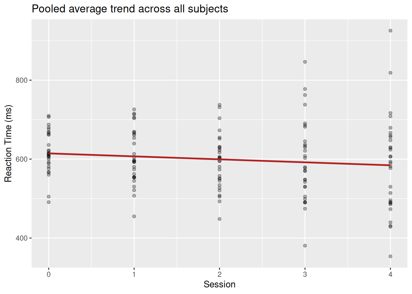
Generally, our sample shows the following trend at the group-level:
Code
sim_data |>ggplot(aes(session, reaction_time)) +geom_point(alpha =0.3) +geom_smooth(method ="lm", formula ='y ~ x', color ="firebrick", se =FALSE) +labs(title ="Pooled average trend across all subjects",x ="Session", y ="Reaction Time (ms)")
The ANOVA approach (full pooling)
What happens when we ignore subjects altogether?
Before diving into mixed models, let’s start with a simple linear model — the kind you’d use in a basic ANOVA-style analysis. This model assumes complete pooling, meaning all subjects are treated as coming from the same population with no individual differences.
Call:
lm(formula = reaction_time ~ 1 + session, data = sim_data)

Residuals:
    Min      1Q  Median      3Q     Max
-230.76  -53.64   -3.20   52.50  341.12

Coefficients:
            Estimate Std. Error t value Pr(>|t|)
(Intercept)  614.455     12.161  50.525   <2e-16 ***
session       -7.529      4.965  -1.516    0.132
---
Signif. codes:  0 '***' 0.001 '**' 0.01 '*' 0.05 '.' 0.1 ' ' 1

Residual standard error: 85.99 on 148 degrees of freedom
Multiple R-squared:  0.0153,    Adjusted R-squared:  0.008646
F-statistic: 2.299 on 1 and 148 DF,  p-value: 0.1316
This model estimates a single intercept (baseline reaction time) and a single slope (learning rate) for everyone. It completely ignores the fact that each participant provides multiple data points.
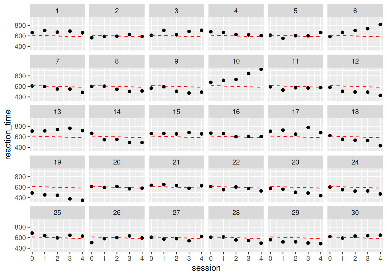
…Here is the model prediction - notice how every participant is assumed to have the same initial value and linear trajectory. This is due to pooling, an assumption from ANOVA. …
Let’s overlay the model predictions onto each subject’s data:
As you can see, the red dashed line is identical across all panels. That’s because the model assumes all participants behave the same — same starting point, same rate of learning. It completely ignores the fact that participants vary in their baseline speed and how much they improve. This is the statistical assumption behind traditional ANOVA: everyone is treated as identical except for random noise.
The elusive discussion of responders/non-responders
At first glance, you might look at this and say:
“Ah, some people are improving, others aren’t — we have responders and non-responders!”
But that interpretation would be misleading here. This model can’t tell you who is improving — it just imposes the same trend on everyone. The differences you see are purely residuals (errors), not modeled variation.
Modeling variation by treating every participant as their own experiment (no pooling)
Modeling each participant separately (no pooling)
To better capture individual differences, we can treat each participant as their own mini-experiment. This means fitting a separate linear regression model for each subject, without assuming any shared parameters. This is the no pooling approach — the opposite extreme of the ANOVA model.
… If we want to be more sensitive to individual variability, we need to allow participants to be modeled more individually. This can be done by computing linear regression for each participant, treating them as individual cases with no overlap. …
There is this need function in lme4 that does this for you:
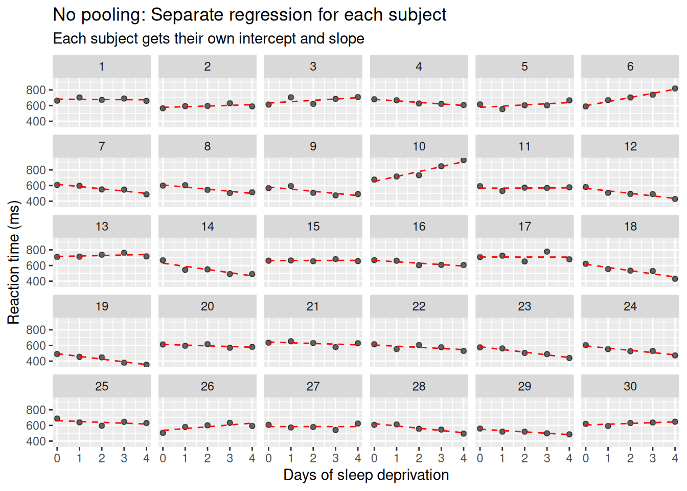
sim_data |>ggplot(aes(session, reaction_time, group=subject)) +facet_wrap(~subject, ncol=6) +geom_point(alpha =0.6) +geom_line(aes(y =fitted(no_pooling)), color ="red", linetype ="dashed") +labs(title ="No pooling: Separate regression for each subject",subtitle ="Each subject gets their own intercept and slope",x ="Days of sleep deprivation", y ="Reaction time (ms)") +scale_x_continuous(limits=c(0, 4),breaks=c(0:4))
What does this show? Now, each subject has their own line, fitted independently from the others.
This approach fully respects subject-level variation — but at a cost.
Although no pooling gives us maximum flexibility, it also comes with trade-offs:
It doesn’t borrow strength across subjects. If someone has noisy data, their slope might be wildly off.
There’s no generalization — you can’t talk about an average effect across subjects, only 30 separate stories.
In small datasets (as is common in biomedical studies), this often leads to unstable estimates.
Key point No pooling shows us the raw heterogeneity in slopes and intercepts — but it doesn’t help us make population-level inferences or control for noise. We need something in between.
What if we want to both model individual differences and estimate a general trend across subjects?
Multi’level regression (partial pooling)
This is where things get interesting — we’re now ready to bridge the gap between the overly simplistic (ANOVA) and the overly fragmented (no pooling) approaches.
Partial pooling with random intercepts
The random intercept model is the first step toward balancing the extremes of full pooling and no pooling.
We acknowledge that subjects vary in their baseline levels (reaction times), but we still assume they share a common trend — in this case, how their reaction times change over sessions.
The following code chunk and plot is based on a mixed-effects model: it includes both fixed effects (shared across all subjects) and random effects (varying by subject).
Linear mixed model fit by REML ['lmerMod']
Formula: reaction_time ~ 1 + session + (1 | subject)
   Data: sim_data

REML criterion at convergence: 1639.3

Scaled residuals:
    Min      1Q  Median      3Q     Max
-2.6679 -0.4728 -0.0547  0.4959  3.8078

Random effects:
 Groups   Name        Variance Std.Dev.
 subject  (Intercept) 5402     73.50
 Residual             2103     45.85
Number of obs: 150, groups:  subject, 30

Fixed effects:
            Estimate Std. Error t value
(Intercept)  614.455     14.904  41.229
session       -7.529      2.647  -2.844

Correlation of Fixed Effects:
        (Intr)
session -0.355
Code
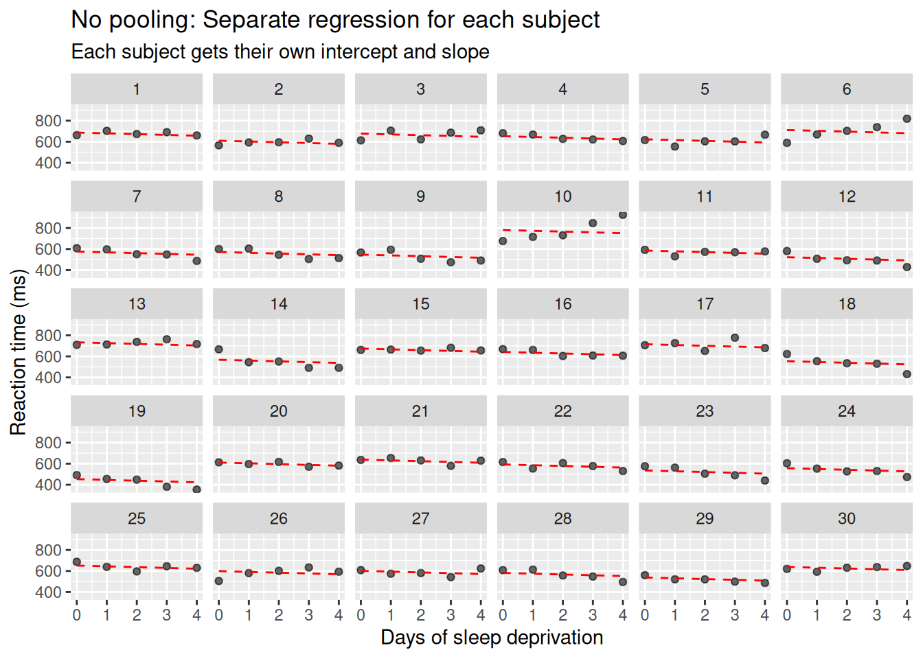
sim_data |>ggplot(aes(session, reaction_time, group=subject)) +facet_wrap(~subject, ncol=6) +geom_point(alpha =0.6) +geom_line(aes(y =fitted(RI_only)), color ="red", linetype ="dashed") +labs(title ="No pooling: Separate regression for each subject",subtitle ="Each subject gets their own intercept and slope",x ="Days of sleep deprivation", y ="Reaction time (ms)") +scale_x_continuous(limits=c(0, 4),breaks=c(0:4))
What does this model assume?
Each subject has their own intercept (baseline reaction time), but they all share the same learning (or fatigue) slope. This is often better than full pooling, because it accounts for subject differences in level — but it may still be too rigid if slopes really do vary. If some participants improve rapidly while others don’t, a fixed slope assumption can:
Underestimate uncertainty in the group trend,
Bias the estimate of the average slope,
Lead to false positives (thinking there’s a trend when it’s driven by a few outliers),
Mislead clinical interpretations — e.g. calling someone a “responder” when it’s just model misfit.
Limitations of Random Intercept Models in Clinical Inference
In applied biomedical and clinical research, it is common to assess whether individuals vary in their response to an intervention or over repeated measurements. A random intercept model allows for differences in baseline levels between participants but assumes that all individuals share a common rate of change (i.e., a fixed slope).
This assumption can be problematic. If individuals truly differ in their trajectories—such as some improving and others not—then forcing a single slope across all subjects may misattribute systematic variation to residual noise. This can result in biased fixed-effect estimates and inflated residual variance, especially if a small number of participants deviate substantially from the average trend.
In such cases, interpreting individual deviations from the model as evidence of “responders” or “non-responders” can be misleading. These deviations may reflect model misfit rather than genuine subject-specific effects.
Current consensus in the statistical literature supports the use of random slope models when there is theoretical or empirical justification for individual differences in change over time. These models can account for both baseline heterogeneity and subject-specific trends, offering more accurate and generalizable inference (Gelman & Hill, 2007; Barr et al., 2013).
Random slopes:
To account for individual differences not only in baseline levels but also in rates of change, we now extend the model to include random slopes. This allows each subject to have their own intercept and their own slope with respect to session.
Linear mixed model fit by REML ['lmerMod']
Formula: reaction_time ~ 1 + session + (session | subject)
   Data: sim_data

REML criterion at convergence: 1550.6

Scaled residuals:
     Min       1Q   Median       3Q      Max
-2.06073 -0.52670 -0.00823  0.53737  2.59156

Random effects:
 Groups   Name        Variance Std.Dev. Corr
 subject  (Intercept) 2090.4   45.72
          session      565.9   23.79    0.30
 Residual              723.6   26.90
Number of obs: 150, groups:  subject, 30

Fixed effects:
            Estimate Std. Error t value
(Intercept)  614.455      9.174  66.981
session       -7.529      4.612  -1.632

Correlation of Fixed Effects:
        (Intr)
session 0.147
This model assumes that:
The intercepts vary by subject (baseline differences),
The slopes also vary by subject (individual learning rates),
And these random effects can be correlated (e.g., subjects with higher baselines may also learn faster or slower).
By allowing for both random intercepts and random slopes, we acknowledge that participants may respond differently over time — something particularly important in biomedical and behavioral research, where inter-individual variability is the norm rather than the exception.
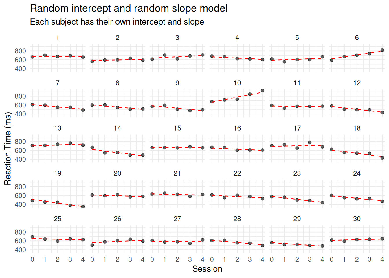
Let’s visualize the fitted lines from this model:
Code
sim_data$RI_RS_fitted <-predict(RI_RS_corr)sim_data |>ggplot(aes(x = session, y = reaction_time, group = subject)) +facet_wrap(~ subject, ncol =6) +geom_point(alpha =0.6) +geom_line(aes(y = RI_RS_fitted), color ="red", linetype ="dashed") +labs(title ="Random intercept and random slope model",subtitle ="Each subject has their own intercept and slope",x ="Session", y ="Reaction Time (ms)") +scale_x_continuous(limits =c(0, 4), breaks =0:4) +theme_minimal()
Random slope models can:
Improve model fit by accounting for structured variability,
Produce more accurate estimates of population-level effects,
Reduce the risk of false positives or negatives due to mis-specified structure,
And provide a framework for investigating individual differences in trajectories — a key concern in many health-related studies.
This approach represents what is often called partial pooling: estimates are informed both by the individual subject’s data and by the group-level trend, leading to more stable and interpretable inference, especially in small to moderate samples.
Comparing models: Do random slopes improve fit?
We now compare two models:
One that allows subjects to differ only in their baseline level (random intercept),
And another that also allows them to differ in their rate of change over sessions (random slope).
Using the Akaike Information Criterion, we can assess model fit:
Using the REML criterion (restricted maximum likelihood), we can assess model fit:
Model
Model REML criterion
Random intercept only
1639.3
Random intercept + random slope
1550.6
Lower AIC values indicate better fit. Here, the random slope model shows a substantially lower AIC, suggesting that accounting for individual variability in slopes improves model fit.
If we wanted to formally test whether adding random slopes improves the model, we could refit both models using maximum likelihood (ML) and then conduct a likelihood ratio test:
This test examines whether the added complexity (the subject-specific slopes and the correlation between random intercept and random slope) is justified by a significantly better fit.
The model with random slopes:
Fits the data substantially better (lower REML),
Produces more conservative fixed-effect estimates (larger SE, smaller t),
Accounts for the correlation between intercepts and slopes across individuals (here: +0.30),
And reduces residual variance (from ~2103 to ~723), indicating that more of the variability is now captured by structured random effects.
This supports the idea that in biomedical or behavioral data — where individual responses often differ — a random intercept-only model may be too restrictive and lead to misleading fixed-effect conclusions.
Interpreting the Random Effects
The random intercept + slope model with added correlation term gives us valuable insight into the structure of variability in our data — not just whether an effect exists on average, but how consistent it is across individuals.
From the model output:
Code
summary(RI_RS_corr)
Linear mixed model fit by REML ['lmerMod']
Formula: reaction_time ~ 1 + session + (session | subject)
   Data: sim_data

REML criterion at convergence: 1550.6

Scaled residuals:
     Min       1Q   Median       3Q      Max
-2.06073 -0.52670 -0.00823  0.53737  2.59156

Random effects:
 Groups   Name        Variance Std.Dev. Corr
 subject  (Intercept) 2090.4   45.72
          session      565.9   23.79    0.30
 Residual              723.6   26.90
Number of obs: 150, groups:  subject, 30

Fixed effects:
            Estimate Std. Error t value
(Intercept)  614.455      9.174  66.981
session       -7.529      4.612  -1.632

Correlation of Fixed Effects:
        (Intr)
session 0.147
Baseline (Intercept) Variability The standard deviation of the intercepts is 45.72 ms, indicating substantial between-subject differences in baseline reaction times. This is expected in behavioral or clinical data, where individuals differ due to prior experience, cognitive ability, or other latent traits.
Slope (Session Effect) Variability The standard deviation of the random slopes is 23.79 ms, meaning that individuals differ notably in how their reaction times change over sessions — some improve sharply, others remain flat or even worsen slightly. This heterogeneity is clinically relevant and would be obscured by models that assume a common slope.
Correlation Between Intercepts and Slopes The correlation between intercepts and slopes is +0.30. This suggests a weak-to-moderate tendency for participants with higher baseline reaction times to show steeper improvements (more negative slopes). While not strong, this association may point to individual differences in learning potential — e.g., those starting slower have more room to improve.
This can be visualized:
Code
sim_data |> dplyr::mutate(improving = slope_re <0) |>ggplot(aes(y=reaction_time, x=session, color = improving)) +scale_color_manual(values =c("TRUE"="blue", "FALSE"="gray")) +facet_wrap(~ subject, ncol=6) +geom_point() +geom_line() +geom_hline(yintercept=mean(subset(sim_data,session==1)$reaction_time)) +scale_x_continuous(limits=c(0, 4),breaks=c(0:4)) +labs(x ="Session", y ="Reaction Time (ms)",title ="Individual learning trajectories across sessions")
Why this matters
The comparison to a simpler model (with only random intercepts) showed that assuming a shared slope across participants can lead to misleading fixed-effect estimates. Notice that while the estimate is identical, the standard error of the estimate increased almost two-fold, yielding a lower test statistic.
Model
Fixed Effect
Estimate
Std. Error
t value
RI_only
session
-7.53
2.65
-2.84
RI_RS_corr
session
-7.53
4.61
-1.63
The estimate is identical in both models, but the standard error increases substantially in the random slope model. This reflects how the RI-only model underestimates uncertainty by ignoring individual variability in slopes. Consequently, the t-value drops from a statistically suggestive level (–2.84) to a more cautious level (–1.63), demonstrating the importance of correctly specifying random effects.
The average effect remains the same, but the uncertainty increases, because the model properly attributes some of the variation to individual differences.
This is exactly what Gelman & Hill (2007) and Barr et al. (2013) argue: failing to include justified random slopes can inflate confidence in fixed effects — potentially leading to spurious conclusions.
Key points:
By modeling random slopes: - We acknowledge that people learn differently over time, - We prevent overconfident or misleading group-level inferences, - And we gain access to rich insights about how variability in individual responses relates to baseline ability.
This modeling approach helps move us from averages to individuals, which is crucial in many health, cognitive, and behavioral domains.
Take-away message:
So, what did we learn from all this?
We explored a progression of modeling approaches:
From ANOVA-style pooling,
to mass regression (no pooling),
then to partial pooling with a random intercept,
and finally to a model with both random intercepts and slopes, including their correlation.
Each step improved the model fit. But here’s the key insight: Only the model with random slopes gave us a trustworthy picture of individual differences.
The random intercept-only model, while tempting in its simplicity, produced misleading results. Specifically, it underestimated standard errors, leading to inflated Type I error rates. That’s not just a technical detail — it can fundamentally distort scientific conclusions, especially in clinical or psychological studies where understanding who improves and who doesn’t is crucial.
So, if you’re working with repeated measures or hierarchical data and you care about individual variability, responder/non-responder patterns, or generalization, don’t stop at random intercepts.
Modeling the variance-covariance structure of the specific data set (i.e. random terms of the mixed-effect model) aren’t just a technical flourish — they’re essential for honest modeling.
While random intercept models are within the class of linear mixed-effect models, they are often difficult to find use cases for within cognitive neuroscience experiments.
While accounting for individual starting differences is a step up from the ANOVA approach, it still assumes no variability between participants.
Fitting mass linear models (no pooling) overcomes this problem. However, researchers often aim to generalize and make population-based conclusions. It is therefore not optimal for this use case.
Linear mixed-effect models that are modeled appropriately to a specific data set is a great approach (partial-pooling). However, they quickly become tricky to set up when there are multiple predictors, groups, covariates, and especially interactions.