Why random slopes matters…

… and why random intercepts are often not enough

Using lme4, I show why random slopes is often needed in biomedical research and experiments

Multi-level models and why random slopes matter

In this post, we’ll discuss why random slopes are often of special concern in health science data and biometrics. We will use lme4 and ggplot2 to do so. The data set we’ll use to demonstrate this comes from …

Loading required package: Matrix

Attaching package: 'dplyr'

The following objects are masked from 'package:stats':

    filter, lag

The following objects are masked from 'package:base':

    intersect, setdiff, setequal, union

Generating our data set:

set.seed(314)

# Parameters
n_subjects <- 30
n_sessions <- 5

# Fixed effect of session: general learning effect
beta_0 <- 600   # Average baseline RT in ms
beta_1 <- -10   # Average decrease in RT per session

# Random effects: standard deviations
sd_intercept <- 50    # SD of baseline RTs across subjects
sd_slope     <- 25    # SD of learning rates (slopes)
rho          <- 0.2   # Correlation between intercepts and slopes

# Within-subject residual error
sigma_error <- 30

# Construct subject-level random effects (correlated)
subject_re <- MASS::mvrnorm(
  n = n_subjects,
  mu = c(0, 0),
  Sigma = matrix(c(sd_intercept^2, rho*sd_intercept*sd_slope,
                   rho*sd_intercept*sd_slope, sd_slope^2), 2)
) |> 
  as.data.frame() |>
  setNames(c("intercept_re", "slope_re")) |>
  dplyr::mutate(subject = factor(1:n_subjects))

# Create session vector repeated for each subject
session <- rep(0:(n_sessions - 1), times = n_subjects)

# Repeat subject IDs for each session
subject <- rep(subject_re$subject, each = n_sessions)

# Join the random effects
sim_data <- tibble::tibble(subject = subject, session = session) |>
  dplyr::left_join(subject_re, by = "subject") |>
  dplyr::mutate(
    reaction_time = beta_0 + intercept_re +
                    (beta_1 + slope_re) * session +
                    rnorm(dplyr::n(), mean = 0, sd = sigma_error)
  )

# View a few rows
head(sim_data)

# A tibble: 6 × 5
  subject session intercept_re slope_re reaction_time
  <fct>     <int>        <dbl>    <dbl>         <dbl>
1 1             0         63.5     14.4          663.
2 1             1         63.5     14.4          703.
3 1             2         63.5     14.4          673.
4 1             3         63.5     14.4          691.
5 1             4         63.5     14.4          660.
6 2             0        -39.0     15.7          566.

A brief look at the data:

str(sim_data) # for more info, consult ?lme4::sleepstudy for the lme4 documentation

tibble [150 × 5] (S3: tbl_df/tbl/data.frame)
 $ subject      : Factor w/ 30 levels "1","2","3","4",..: 1 1 1 1 1 2 2 2 2 2 ...
 $ session      : int [1:150] 0 1 2 3 4 0 1 2 3 4 ...
 $ intercept_re : num [1:150] 63.5 63.5 63.5 63.5 63.5 ...
 $ slope_re     : num [1:150] 14.4 14.4 14.4 14.4 14.4 ...
 $ reaction_time: num [1:150] 663 703 673 691 660 ...

sim_data |> 
  ggplot(aes(y=reaction_time, x=session)) +
  facet_wrap(~ subject, ncol=6) +
  geom_point() +
  geom_line() +
  scale_x_continuous(limits=c(0, 5),breaks=c(0:5))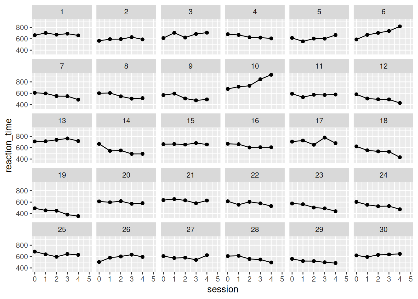

RI_only <- lme4::lmer(reaction_time ~ 1 + session + (1 | subject), sim_data)
summary(RI_only)

Linear mixed model fit by REML ['lmerMod']
Formula: reaction_time ~ 1 + session + (1 | subject)
   Data: sim_data

REML criterion at convergence: 1639.3

Scaled residuals: 
    Min      1Q  Median      3Q     Max 
-2.6679 -0.4728 -0.0547  0.4959  3.8078 

Random effects:
 Groups   Name        Variance Std.Dev.
 subject  (Intercept) 5402     73.50   
 Residual             2103     45.85   
Number of obs: 150, groups:  subject, 30

Fixed effects:
            Estimate Std. Error t value
(Intercept)  614.455     14.904  41.229
session       -7.529      2.647  -2.844

Correlation of Fixed Effects:
        (Intr)
session -0.355

2 * pnorm(-1.744)

[1] 0.08115909

RI_RS_corr <- lme4::lmer(reaction_time ~ 1 + session + (session | subject), sim_data)
summary(RI_RS_corr)

Linear mixed model fit by REML ['lmerMod']
Formula: reaction_time ~ 1 + session + (session | subject)
   Data: sim_data

REML criterion at convergence: 1550.6

Scaled residuals: 
     Min       1Q   Median       3Q      Max 
-2.06073 -0.52670 -0.00823  0.53737  2.59156 

Random effects:
 Groups   Name        Variance Std.Dev. Corr 
 subject  (Intercept) 2090.4   45.72         
          session      565.9   23.79    0.30 
 Residual              723.6   26.90         
Number of obs: 150, groups:  subject, 30

Fixed effects:
            Estimate Std. Error t value
(Intercept)  614.455      9.174  66.981
session       -7.529      4.612  -1.632

Correlation of Fixed Effects:
        (Intr)
session 0.147 

2 * pnorm(-1.428)

[1] 0.1532919

sleepstudy |> 
  ggplot(aes(y=Reaction, x=Days)) +
  facet_wrap(~ Subject, ncol=6) +
  geom_point() +
  geom_line() +
  scale_x_continuous(limits=c(0, 9),breaks=c(0:9))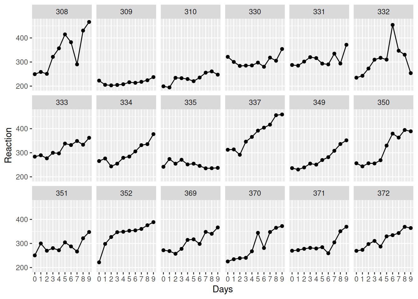

The ANOVA approach (full pooling)

anova_approach <- lm(Reaction ~ 1 + Days, sleepstudy)
summary(anova_approach)

Call:
lm(formula = Reaction ~ 1 + Days, data = sleepstudy)

Residuals:
     Min       1Q   Median       3Q      Max 
-110.848  -27.483    1.546   26.142  139.953 

Coefficients:
            Estimate Std. Error t value Pr(>|t|)    
(Intercept)  251.405      6.610  38.033  < 2e-16 ***
Days          10.467      1.238   8.454 9.89e-15 ***
---
Signif. codes:  0 '***' 0.001 '**' 0.01 '*' 0.05 '.' 0.1 ' ' 1

Residual standard error: 47.71 on 178 degrees of freedom
Multiple R-squared:  0.2865,    Adjusted R-squared:  0.2825 
F-statistic: 71.46 on 1 and 178 DF,  p-value: 9.894e-15

Here is the model prediction - notice how every participant is assumed to have the same initial value and linear trajectory. This is due to pooling, an assumption from ANOVA.

ggplot(sleepstudy, aes(Days, Reaction, group=Subject)) + 
  facet_wrap(~Subject, ncol=6) +
  geom_point() + 
  geom_line(aes(y=fitted(anova_approach)), linetype=2, color = "red") + 
  scale_x_continuous(limits=c(0, 9),breaks=c(0:9))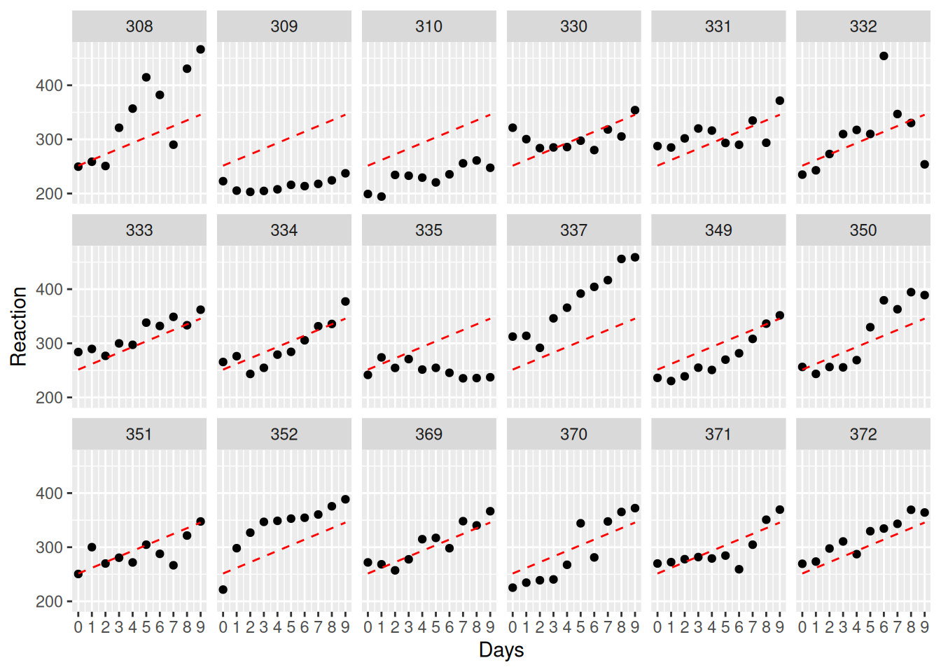

No pooling - treating every participant as their own experiment…

If we want to be more sensitive to individual variability, we need to allow participants to be modeled more individually. This can be done by computing linear regression for each participant, treating them as individual cases with no overlap.

no_pooling <- lmList(Reaction ~ Days | Subject, sleepstudy)
summary(no_pooling)

Call:
  Model: Reaction ~ Days | NULL 
   Data: sleepstudy 

Coefficients:
   (Intercept) 
    Estimate Std. Error  t value     Pr(>|t|)
308 244.1927   15.04169 16.23439 2.419368e-34
309 205.0549   15.04169 13.63244 1.067180e-27
310 203.4842   15.04169 13.52802 1.993900e-27
330 289.6851   15.04169 19.25882 1.122068e-41
331 285.7390   15.04169 18.99647 4.646933e-41
332 264.2516   15.04169 17.56795 1.236403e-37
333 275.0191   15.04169 18.28379 2.303436e-39
334 240.1629   15.04169 15.96649 1.135574e-33
335 263.0347   15.04169 17.48705 1.946826e-37
337 290.1041   15.04169 19.28667 9.653936e-42
349 215.1118   15.04169 14.30104 1.983389e-29
350 225.8346   15.04169 15.01391 2.939145e-31
351 261.1470   15.04169 17.36155 3.943049e-37
352 276.3721   15.04169 18.37374 1.402577e-39
369 254.9681   15.04169 16.95077 4.023936e-36
370 210.4491   15.04169 13.99106 1.253782e-28
371 253.6360   15.04169 16.86221 6.656453e-36
372 267.0448   15.04169 17.75365 4.373979e-38
   Days 
     Estimate Std. Error    t value     Pr(>|t|)
308 21.764702   2.817566  7.7246464 1.741840e-12
309  2.261785   2.817566  0.8027444 4.234454e-01
310  6.114899   2.817566  2.1702769 3.162541e-02
330  3.008073   2.817566  1.0676139 2.874813e-01
331  5.266019   2.817566  1.8689956 6.365457e-02
332  9.566768   2.817566  3.3954013 8.857738e-04
333  9.142045   2.817566  3.2446604 1.462120e-03
334 12.253141   2.817566  4.3488388 2.574673e-05
335 -2.881034   2.817566 -1.0225257 3.082469e-01
337 19.025974   2.817566  6.7526272 3.315759e-10
349 13.493933   2.817566  4.7892159 4.115160e-06
350 19.504017   2.817566  6.9222924 1.356856e-10
351  6.433498   2.817566  2.2833528 2.387301e-02
352 13.566549   2.817566  4.8149886 3.683105e-06
369 11.348109   2.817566  4.0276282 9.081880e-05
370 18.056151   2.817566  6.4084212 1.964766e-09
371  9.188445   2.817566  3.2611283 1.385338e-03
372 11.298073   2.817566  4.0098697 9.718197e-05

Residual standard error: 25.59182 on 144 degrees of freedom

ggplot(sleepstudy, aes(Days, Reaction, group=Subject)) + 
  facet_wrap(~Subject, ncol=6) +
  geom_point() + 
  geom_line(aes(y=fitted(no_pooling)), linetype=2, color = "red") + 
  scale_x_continuous(limits=c(0, 9),breaks=c(0:9))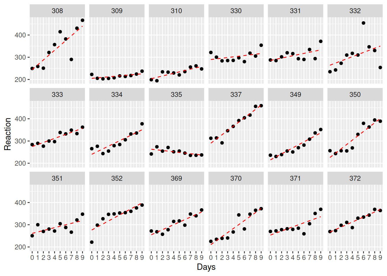

Partial pooling

With random intercept only:

We can relax the assumption of pooling by allowing each participant to have their own intercept.

RI_only <- lmer(Reaction ~ 1 + Days + (1 | Subject), sleepstudy)
summary(RI_only)

Linear mixed model fit by REML ['lmerMod']
Formula: Reaction ~ 1 + Days + (1 | Subject)
   Data: sleepstudy

REML criterion at convergence: 1786.5

Scaled residuals: 
    Min      1Q  Median      3Q     Max 
-3.2257 -0.5529  0.0109  0.5188  4.2506 

Random effects:
 Groups   Name        Variance Std.Dev.
 Subject  (Intercept) 1378.2   37.12   
 Residual              960.5   30.99   
Number of obs: 180, groups:  Subject, 18

Fixed effects:
            Estimate Std. Error t value
(Intercept) 251.4051     9.7467   25.79
Days         10.4673     0.8042   13.02

Correlation of Fixed Effects:
     (Intr)
Days -0.371

Note the fixed effect 10.4673 / 0.8042 = 13.0157921

ggplot(sleepstudy, aes(Days, Reaction, group=Subject)) + 
  facet_wrap(~Subject, ncol=6) +
  geom_point() + 
  geom_line(aes(y=fitted(RI_only)), linetype=2, color = "red") + 
  scale_x_continuous(limits=c(0, 9),breaks=c(0:9))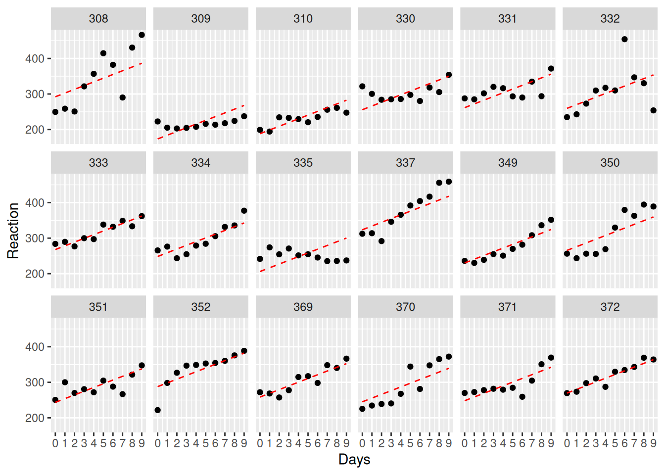

Now with random intercept, random slope, and correlated random terms

RI_RS_corr <- lmer(Reaction ~ 1 + Days + (1 + Days | Subject), sleepstudy)
summary(RI_RS_corr)

Linear mixed model fit by REML ['lmerMod']
Formula: Reaction ~ 1 + Days + (1 + Days | Subject)
   Data: sleepstudy

REML criterion at convergence: 1743.6

Scaled residuals: 
    Min      1Q  Median      3Q     Max 
-3.9536 -0.4634  0.0231  0.4634  5.1793 

Random effects:
 Groups   Name        Variance Std.Dev. Corr 
 Subject  (Intercept) 612.10   24.741        
          Days         35.07    5.922   0.07 
 Residual             654.94   25.592        
Number of obs: 180, groups:  Subject, 18

Fixed effects:
            Estimate Std. Error t value
(Intercept)  251.405      6.825  36.838
Days          10.467      1.546   6.771

Correlation of Fixed Effects:
     (Intr)
Days -0.138

Note the fixed effect 10.467 / 1.546 = 6.7703752

ggplot(sleepstudy, aes(Days, Reaction, group=Subject, colour=Subject)) + 
  facet_wrap(~Subject, ncol=6) +
  geom_point() + 
  geom_line(aes(y=fitted(RI_RS_corr)), linetype=2, color = "red") + 
  scale_x_continuous(limits=c(0, 9),breaks=c(0:9))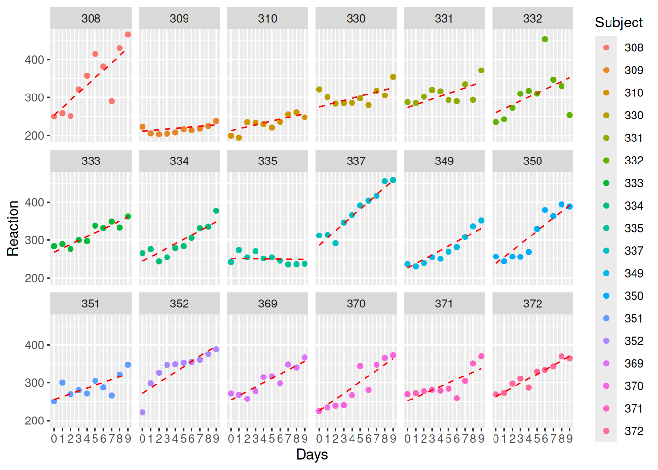

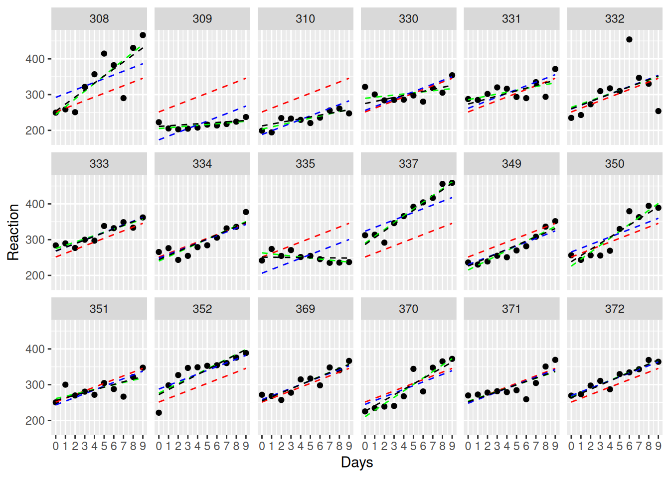
Comparing model predictions

ggplot(sleepstudy, aes(Days, Reaction, group=Subject)) + 
  facet_wrap(~Subject, ncol=6) +
  geom_point() + 
  geom_line(aes(y=fitted(anova_approach)), linetype=2, color = "red") + 
  geom_line(aes(y=fitted(no_pooling)), linetype=2, color = "green") + 
  geom_line(aes(y=fitted(RI_only)), linetype=2, color = "blue") + 
  geom_line(aes(y=fitted(RI_RS_corr)), linetype=2, color = "black") +
  scale_x_continuous(limits=c(0, 9),breaks=c(0:9))

Conclusions

• While random intercept models are within the class of linear mixed-effect models, they are often difficult to find use cases for within cognitive neuroscience experiments.
• While accouting for individual starting differences is a set up from the ANOVA approach, it still assumes no variability between participants.
• Fitting mass linear models (no pooling) overcomes this problem. However, researchers often aim to generalize and make population-based conclusions. It is therefore not optimal for this use case.
• Linear mixed-effect models that are modeled appropriately to a specific data set is a great approach (partial-pooling). However, they quickly become tricky to set up when there are multiple predictors, groups, covariates, and especially interactions.