Why be a Bayesian

A non-technical introduction to the Bayesian approach

Bayesian inference is not only elegant and intuitive, but also helpful for overcoming common challenges with data from the life sciences

Slides

NoteTeacher note

The slides contain speaking notes that you can view by pressing ‘S’ on the keyboard.

Why be a Bayesian?

There are many reasons to be a Bayesian.

What is the alternative?

Frequentist statistics

Is there a fight?

No! That fight ended in the 90’s

When to use Frequentist and when to use Bayesian approaches?

Frequentist are often sufficient and comparable to Bayesian stats.

But sometimes, they are very different!

# install.packages(c("MASS", "rstanarm", "tidyverse"))

library(MASS)
library(rstanarm)

Loading required package: Rcpp

This is rstanarm version 2.32.2

- See https://mc-stan.org/rstanarm/articles/priors for changes to default priors!

- Default priors may change, so it's safest to specify priors, even if equivalent to the defaults.

- For execution on a local, multicore CPU with excess RAM we recommend calling

  options(mc.cores = parallel::detectCores())

library(tidyverse)

── Attaching core tidyverse packages ──────────────────────── tidyverse 2.0.0 ──
✔ dplyr     1.2.1     ✔ readr     2.2.0
✔ forcats   1.0.1     ✔ stringr   1.6.0
✔ ggplot2   4.0.3     ✔ tibble    3.3.1
✔ lubridate 1.9.5     ✔ tidyr     1.3.2
✔ purrr     1.2.2     

── Conflicts ────────────────────────────────────────── tidyverse_conflicts() ──
✖ dplyr::filter() masks stats::filter()
✖ dplyr::lag()    masks stats::lag()
✖ dplyr::select() masks MASS::select()
ℹ Use the conflicted package (<http://conflicted.r-lib.org/>) to force all conflicts to become errors

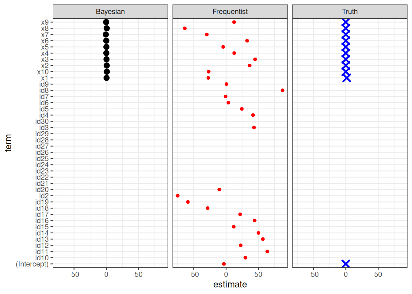
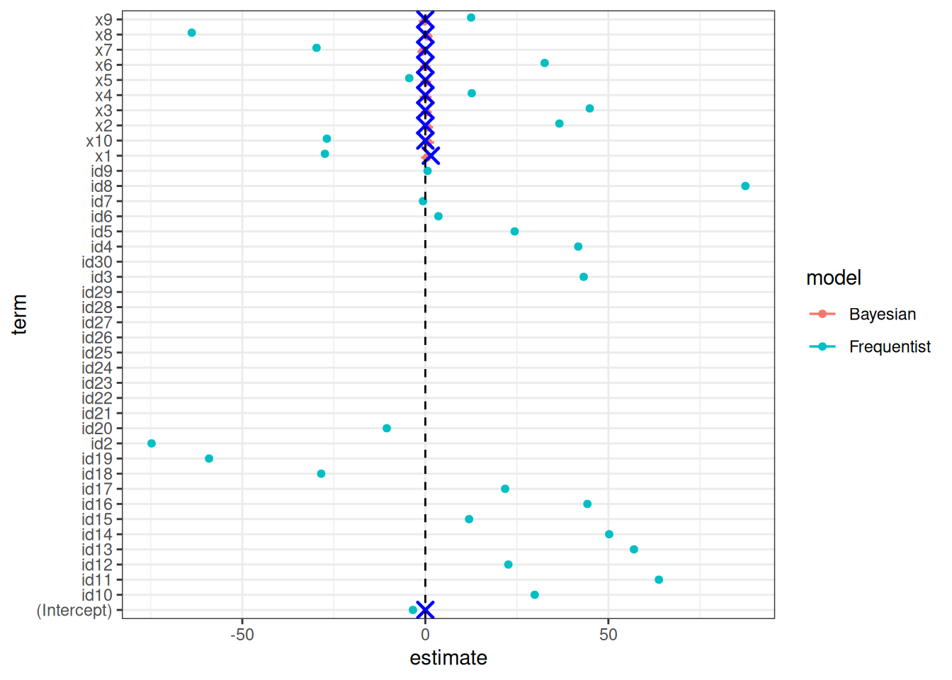
set.seed(12)

# -----------------------------
# Simulate correlated predictors
# -----------------------------

n <- 30
p <- 10

Sigma <- matrix(0.9, p, p)
diag(Sigma) <- 1

X <- MASS::mvrnorm(n, mu = rep(0, p), Sigma = Sigma)

colnames(X) <- paste0("x", 1:p)

# True data-generating process:
# only x1 matters

beta_true <- c(1.5, rep(0, p - 1))

y <- X %*% beta_true + rnorm(n, 0, 2)

dat <- data.frame(y, X, id = 1:n)
dat <- dat |>
  dplyr::mutate(
    id = as.factor(id)
  )

dat_long <- dat |>
  tidyr::pivot_longer(
    cols = starts_with("x"),
    names_to = "predictor",
    values_to = "value",
  )

# -----------------------------
# Frequentist OLS
# -----------------------------

fit_lm <- lm(y ~ ., data = dat)
fit_lm_long <- lm(y ~ ., data = dat_long)

summary(fit_lm)

Call:
lm(formula = y ~ ., data = dat)

Residuals:
ALL 30 residuals are 0: no residual degrees of freedom!

Coefficients: (10 not defined because of singularities)
            Estimate Std. Error t value Pr(>|t|)
(Intercept)  -3.3873        NaN     NaN      NaN
x1          -27.4343        NaN     NaN      NaN
x2           36.6169        NaN     NaN      NaN
x3           44.9134        NaN     NaN      NaN
x4           12.6781        NaN     NaN      NaN
x5           -4.3991        NaN     NaN      NaN
x6           32.5898        NaN     NaN      NaN
x7          -29.7243        NaN     NaN      NaN
x8          -63.8061        NaN     NaN      NaN
x9           12.4932        NaN     NaN      NaN
x10         -26.9036        NaN     NaN      NaN
id2         -74.7875        NaN     NaN      NaN
id3          43.2553        NaN     NaN      NaN
id4          41.7687        NaN     NaN      NaN
id5          24.3886        NaN     NaN      NaN
id6           3.5718        NaN     NaN      NaN
id7          -0.6418        NaN     NaN      NaN
id8          87.4302        NaN     NaN      NaN
id9           0.6060        NaN     NaN      NaN
id10         29.8794        NaN     NaN      NaN
id11         63.7978        NaN     NaN      NaN
id12         22.6777        NaN     NaN      NaN
id13         56.9841        NaN     NaN      NaN
id14         50.2156        NaN     NaN      NaN
id15         11.9500        NaN     NaN      NaN
id16         44.2689        NaN     NaN      NaN
id17         21.7949        NaN     NaN      NaN
id18        -28.4541        NaN     NaN      NaN
id19        -59.0872        NaN     NaN      NaN
id20        -10.5432        NaN     NaN      NaN
id21              NA         NA      NA       NA
id22              NA         NA      NA       NA
id23              NA         NA      NA       NA
id24              NA         NA      NA       NA
id25              NA         NA      NA       NA
id26              NA         NA      NA       NA
id27              NA         NA      NA       NA
id28              NA         NA      NA       NA
id29              NA         NA      NA       NA
id30              NA         NA      NA       NA

Residual standard error: NaN on 0 degrees of freedom
Multiple R-squared:      1, Adjusted R-squared:    NaN 
F-statistic:   NaN on 29 and 0 DF,  p-value: NA

# -----------------------------
# Bayesian regression
# -----------------------------

fit_bayes <- rstanarm::stan_glm(
  y ~ .,
  data = dat,
  prior = rstanarm::normal(0, 1),
  prior_intercept = rstanarm::normal(0, 5),
  chains = 4,
  iter = 2000,
  refresh = 0
)

print(fit_bayes, digits = 2)

stan_glm
 family:       gaussian [identity]
 formula:      y ~ .
 observations: 30
 predictors:   40
------
            Median MAD_SD
(Intercept) -0.07   0.37 
x1           0.40   0.82 
x2           0.63   0.80 
x3           0.30   0.76 
x4           0.09   0.78 
x5           0.17   0.74 
x6          -0.02   0.72 
x7          -0.79   0.71 
x8           0.65   0.68 
x9          -0.24   0.79 
x10          0.79   0.81 
id2         -0.19   0.90 
id3         -0.61   0.89 
id4         -0.23   0.92 
id5          0.65   0.93 
id6          0.51   0.88 
id7         -0.05   0.89 
id8          0.13   0.91 
id9          0.94   0.91 
id10        -0.01   0.91 
id11         0.06   0.88 
id12         0.02   0.89 
id13         0.27   0.90 
id14         0.50   0.89 
id15        -0.64   0.92 
id16        -0.03   0.88 
id17        -0.55   0.89 
id18         0.07   0.89 
id19        -0.18   0.90 
id20        -0.96   0.90 
id21         0.51   0.89 
id22         0.01   0.89 
id23        -0.55   0.93 
id24         0.22   0.92 
id25        -0.32   0.90 
id26         0.25   0.89 
id27        -0.05   0.90 
id28         0.39   0.90 
id29         0.19   0.88 
id30         0.59   0.91 

Auxiliary parameter(s):
      Median MAD_SD
sigma 1.76   0.32  

------
* For help interpreting the printed output see ?print.stanreg
* For info on the priors used see ?prior_summary.stanreg

fit_bayes |>
  tidybayes::spread_draws(
    #`(Intercept)`,
    `^x\\d+`,
    regex = TRUE
  ) |>
  #tidybayes::median_qi(condition_mean = `(Intercept)` + b, .width = c(.95, .66)) |>
  tidybayes::median_qi(x1, .width = c(.95, .66)) |>
  #ggplot2::ggplot(aes(y = group, x = condition_mean, xmin = .lower, xmax = .upper)) +
  ggplot2::ggplot(aes(y = x1, x = x1, xmin = .lower, xmax = .upper)) +
  ggdist::geom_pointinterval()

####

bayes_draws <- fit_bayes |>
  #tidybayes::spread_draws(`(Intercept)`, `^x\\d+`, regex = TRUE) |>
  tidybayes::spread_draws(`^x\\d+`, regex = TRUE) |>
  tidyr::pivot_longer(
    #cols = c(`(Intercept)`, tidyselect::starts_with("x")),
    cols = tidyselect::starts_with("x"),
    names_to = "term",
    values_to = "estimate"
  ) |>
  dplyr::mutate(model = "Bayesian")


freq_df <- broom::tidy(fit_lm, conf.int = TRUE) |>
  dplyr::select(term, estimate, conf.low, conf.high) |>
  dplyr::mutate(model = "Frequentist")

Warning in qt(a, object$df.residual): NaNs produced

truth_df <- tibble::tibble(
  term = c("(Intercept)", paste0("x", 1:p)),
  truth = c(0, beta_true),
  model = "Truth"
)

ggplot2::ggplot() +

  # Bayesian posterior intervals
  ggdist::stat_pointinterval(
    data = bayes_draws,
    aes(x = estimate, y = term),
    .width = c(.5, .8, .95)
  ) +

  # Frequentist estimates + CI
  ggdist::geom_pointinterval(
    data = freq_df,
    aes(
      x = estimate,
      xmin = conf.low,
      xmax = conf.high,
      y = term
    ),
    color = "red"
  ) +

  # Truth
  ggplot2::geom_point(
    data = truth_df,
    ggplot2::aes(x = truth, y = term),
    color = "blue",
    size = 3,
    shape = 4,
    stroke = 1.5
  ) +

  ggplot2::facet_wrap(~model) +

  ggplot2::theme_bw()

Warning: Removed 40 rows containing missing values or values outside the scale range
(`geom_segment()`).

## other approach

bayes_summary <- bayes_draws |>
  dplyr::group_by(term) |>
  tidybayes::median_qi(estimate, .width = 0.95) |>
  dplyr::transmute(
    term,
    estimate,
    conf.low = .lower,
    conf.high = .upper,
    model = "Bayesian"
  )


freq_plot <- freq_df |>
  dplyr::transmute(
    term,
    estimate,
    conf.low,
    conf.high,
    model = "Frequentist"
  )

plot_df <- dplyr::bind_rows(
  bayes_summary,
  freq_plot
)

ggplot2::ggplot(
  plot_df,
  ggplot2::aes(
    x = estimate,
    y = term,
    color = model
  )
) +

  ggdist::geom_pointinterval(
    ggplot2::aes(
      xmin = conf.low,
      xmax = conf.high
    ),
    position = ggplot2::position_dodge(width = 0.5)
  ) +

  ggplot2::geom_point(
    data = truth_df,
    ggplot2::aes(x = truth, y = term),
    inherit.aes = FALSE,
    color = "blue",
    shape = 4,
    size = 3,
    stroke = 1.2
  ) +

  ggplot2::geom_vline(
    xintercept = 0,
    linetype = 2
  ) +

  ggplot2::theme_bw()

Warning: Removed 40 rows containing missing values or values outside the scale range
(`geom_segment()`).