flowchart LR
    A["1. Scientific question<br/><br/>What happens to P(Y)<br/>when X changes?"]

    A --> B["2. Estimator<br/><br/>logistic regression"]

    B --> C["3. Regression estimate<br/><br/>log-odds"]

    C --> D["4. Quantity to communicate<br/><br/>Probability"]

    D --> E{"5. Who/where are we estimating the effect?"}

    E --> E1["Particular patient"]
    E --> E2["Clinically meaningful<br/>scenario"]
    E --> E3["Average population"]
    E --> E4["Different levels of<br/>an interacting variable"]

    E1 --> F["6. Marginal effects"]
    E2 --> F["6. Marginal effects"]
    E3 --> F["6. Marginal effects"]
    E4 --> F["6. Marginal effects"]

    F --> G["7. Communicate in<br/>clinically meaningful units"]

    style A fill:#E8F1FB,stroke:#3B6EA5,stroke-width:2px
    style B fill:#F3F3F3,stroke:#666,stroke-width:2px
    style C fill:#E8F5E9,stroke:#4C8C4A,stroke-width:2px
    style D fill:#FFF4D6,stroke:#C79A24,stroke-width:2px
    style E fill:#EDE7F6,stroke:#7656A6,stroke-width:2px
    style F fill:#E8F5E9,stroke:#4C8C4A,stroke-width:2px
    style G fill:#DDF3E0,stroke:#3D8B40,stroke-width:3px
15 Marginalizing the problem
15.1 Pree-class Literature
- Marginal effects chatpter 3
-
Marginal effects chatpter 5
- You can skip section 5.4 Uncertainty and 5.5 Test
15.2 Slides
NoteTeacher note
The slides contain speaking notes that you can view by pressing ‘S’ on the keyboard.
15.3 Case session 15: “The odds ratio is 0.65… and so what?”
At the stroke research meeting, the biostatistician puts a slide on the screen.
Thrombectomy vs. no thrombectomy: OR = 0.65
The clinical team pauses.
“That sounds promising,” someone says. “But what does 0.65 actually mean for a patient?”
The analysis comes from an observational study of patients with acute stroke. The outcome is death within one year, and the researchers have fitted a logistic regression model to account for differences between patients who received thrombectomy and those who did not.
The statistician explains that the regression coefficient corresponds to an odds ratio of 0.65.
Another question immediately follows:
“But what we really want to know is whether patients have a lower probability of dying if they receive thrombectomy. Why are we talking about odds?”
Now the room gets filled with discussion.
Suppose 20% of patients in the control group die within one year. What would you actually want to show a clinician—or a patient?
- An odds ratio of 0.65?
- The probability of death under each treatment?
- The absolute difference in probability of death?
- Something else?
And whose probability are we talking about?
- A particular patient with a particular age, diabetes status, and clinical profile?
- An older adult with diabetes?
- The average patient in this study?
- Or the population-level probability we would see if everyone received thrombectomy, compared with what we would see if no one received it?
These are related questions, but they are not the same question. The clinical team decides to work through the problem one scientific question at a time.
- Is thrombectomy associated with a different probability of death?
- Does the effect differ for older adults with diabetes?
- What does the model imply for the average stroke patient?
- What if everyone could participate twice — both in the treatment and the no-treatment group?
The team notices something — the regression model has produced one coefficient, but the researchers have several different scientific questions.
So they ask:
What exactly is the model estimating—and how do we turn that into the quantity we actually want to know?
Your task is to make sure that the quantity we calculate and communicate answers the scientific question we started with.
15.4 Reading Task: Communicating results of regression models
The following text was synthesized from (1) Chapter 2 and adjusted to the topic of the lecture.
A fitted statistical model produces coefficients, but these coefficients are not necessarily the quantities we are scientifically interested in. The estimand is the quantity that answers the research question—the thing we actually want to learn about. A model coefficient, by contrast, is simply a statistical quantity used to represent patterns in the data. It is an abstract output of the model, not medical or clinical information in itself.
For example, a logistic regression produces coefficients on the log-odds scale. Although this may be useful for fitting the model, a log-odds coefficient is often difficult to interpret in practical or clinical terms. It does not directly tell us how a patient’s probability of an outcome changes.
Even probabilities, which are much more familiar, can be surprisingly difficult to interpret. People do not always reason about probabilities intuitively, and research in psychology and behavioral economics has documented many ways in which our judgments about probabilities can be misleading.
This raises an important question: if simple probabilities can be difficult to understand, why make our results even harder to interpret by focusing on quantities such as odds ratios or other model coefficients? The problem becomes even greater with more complicated models involving nonlinear relationships, interactions, random effects, Bayesian models, or machine-learning methods.
The key point is that the model coefficient should usually not be the end of the analysis. We should start with the scientific question and the estimand we want to learn about, and then use the statistical model as a tool for estimating that quantity. When the raw model coefficients are difficult to interpret, we can transform the model results into quantities that are easier to understand and that directly address the research question.
For example, rather than reporting only a logistic regression coefficient or odds ratio, we might report predicted probabilities for clinically meaningful values of the predictors and compare those probabilities. The model is then doing what it is meant to do: providing a statistical representation of the data that helps us learn about a scientifically meaningful quantity.
15.5 Discussion exercise: “What do we actually want to know?”
An observational study retrospecively investigates whether a new treatment reduces the risk of a complication after surgery. The researchers fit a logistic regression model and obtain \(β_1\) (odds ratio) as 0.65 for treatment vs. control.
Discuss with our neighbor:
What is the scientific question? What would you actually want to know about the treatment?
What is the model giving us? What exactly is the odds ratio of 0.65? Is it itself a clinical outcome or something else?
What would be easier to interpret? Imagine the complication occurs in 20% of patients in the control group. What kind of result would you rather show a clinician or patient: the odds ratio, a risk/probability, an absolute risk difference, or something else? Why?
What is the estimand? Try to state, in one sentence, the quantity you would ideally like to learn about.
If the model coefficient is not the scientific answer, what role does the model play?
15.6 Marginalizing the problem - our workflow:
Throughout this session, we’ll use this workflow:
- What is my scientific question — the estimand?
- Choose machinery to model data — the estimator?
- What did the regression estimate — the coefficient?
- What quantity do I actually want to communicate?
- At what values?
- A particular patient?
- A clinically meaningful scenario?
- The average population?
- Different levels of an interacting variable?
- Post-model transformations — the estimate
- Communicate in clinically meaningful units
As shown in Figure 15.1, we move from the scientific question, through the model scale, to a marginal effect on the probability scale.
15.7 Step 1: Four scientific questions
Throughout this session, we’ll tackle four research questions one-by-one:
Does the population who got thrombectory have lower probability of death at 1-year follow-up after stroke compared to the population who did not get thrombectomy?
What is the effect of thrombectory in older adults with diabetes, compared to older adults without diabetes?
What is effect of the average person profile in the sample?
What would be the average probability of death, had all participants received thrombectomy, compared to not receiving it?
WarningFrom model to meaning
In nonlinear models, you cannot generally interpret the regression coefficient as the change in probability.
The purpose of marginaleffects is essentially to help us make this translation: From a fitted generalized model → to quantities that answer the scientific question.
15.7.1 Context
Go ahead and read more about the dataset
?medisr::thrombectomy15.7.2 The estimand
We are interested in the probability of death at 1-year follow-up:
\[ P(death = 1 | X) \]
for an observational study looking at the effect of thrombectomy after stroke:
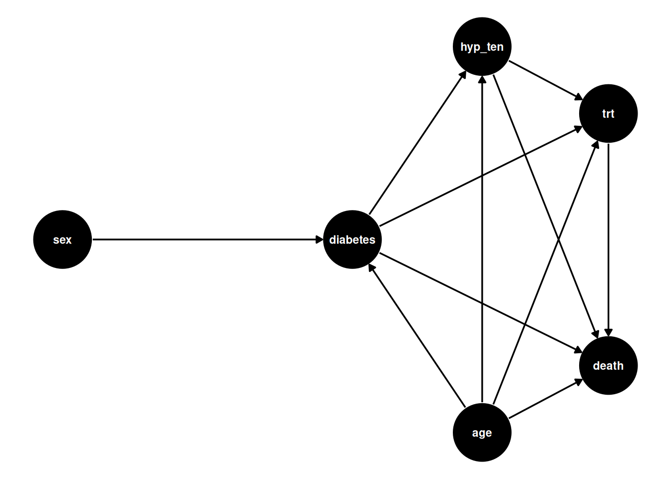
We need to adjust for age, hypertension and diabetes. We will still incl. sex, as the dataset is unbalanced and we want to adjust for that bias.
15.8 Step 2: The estimator
We follow individuals for one year and there is no censoring. The probability of death is relative high (as we’ll see in a minute) and n can be defined as the sample size. So we are able to use logistic regression.
WarningWhat about Poisson regression?
In many ways, this would actually have been the natural choice here, as the dataset has a time aspect and we follow people for longer and some may become censored my migrating etc.
Here, the choice was purely educational — you’ll use poisson regression on the length of stay in the exercises 😄
\[ y_i = Binomial(n,p_i) \\ logit(p_i) = α + βx_i \] where n is the number of observations and p is the probability of death.
The logit function is defined as the log-odds:
\[ logit(p_i) = log(\frac{p_i}{1 - p_i}) \]
The “odds” of an event is just the probability it happens divided by the probability it does not happen. In other words:
\[ log(\frac{p_i}{1 - p_i}) = α + βx_i \] To figure out the definition of p_i, we do some algebra to solve for \(p_i\):
\[ p_i = \frac{exp( α + βx_i)}{1 + exp(α + βx_i)} \] The above function is the logistic
- Note that the log-odds space is linear (what we model)
- The logistic space is the sigmoidal shape (the transformation)
15.8.1 The statistical models
We want to adjust for competing predictors of death and potential counfounders in our model.
\[ logit( \text{death at 1 year followup}) = α + β1_{thrombectomy} + β2_{diabites} + β3_{age} \\ + β4_{hypertention} + β5_{sex} + β6_{thrombectomy×diabites} \\ + β7_{thrombectomy×age} + β8_{thrombectomy×hyptertension} + β9_{thrombectomy×sex} \\ \]
We implement this model in R using glm():
thrombectomy <- medisr::thrombectomy |>
    mutate(death_1year_followup = if_else(time_to_death < 365 & death ==1,1,0),
    age_at_diagnosis = as.numeric(age_at_diagnosis)
    )

th_model <- glm(
  death_1year_followup ~ thrombectomy +
        prior_diabetes +
        age_at_diagnosis +
        prior_hypertention +
        sex +
        thrombectomy:prior_diabetes +
        thrombectomy:age_at_diagnosis +
        thrombectomy:prior_hypertention +
        thrombectomy:sex,
        family = binomial(link = "logit"),
  data = thrombectomy
)
15.9 Step 3: Stock with regression coefficients…
Here’s the model output:
th_model |>
    parameters::parameters(exponentiate=TRUE) |>
    select(Parameter, Coefficient, SE) |>
    rename(Odds_ratio=Coefficient)
# A tibble: 10 × 3
Parameter Odds_ratio SE
<chr> <dbl> <dbl>
1 (Intercept) 0.00182 0.00155
2 thrombectomy 9.06 10.3
3 prior_diabetes 2.70 0.743
4 age_at_diagnosis 1.07 0.0110
5 prior_hypertention 1.48 0.299
6 sex 1.04 0.209
7 thrombectomy:prior_diabetes 1.64 0.760
8 thrombectomy:age_at_diagnosis 0.973 0.0139
9 thrombectomy:prior_hypertention 0.428 0.141
10 thrombectomy:sex 1.34 0.432 Cool, we got an OR = 9.06 for thrombectomy
What does this mean?
15.9.1 Rookie mistake #1
Don’t read this coefficient, thinking it generalizes to the sample!
This sample has odds of 0.00182 for the outcome when thrombectomy = 0 and all other coefficients are 0.
In other words, the intercept describes the model’s baseline odds for a 0-year-old female without diabetes or hypertension, and without thrombectomy. Such a patient didn’t participate in the study. Thus, this is out-of-sample prediction — and a pretty silly and unjustified extrapolation from what we’re trying to answer scientifically here.
The thrombectomy OR of 9.06 means that, holding all the other variables constant, the odds are multiplied by 9.06 when thrombectomy changes from 0 to 1.
15.9.2 Rookie mistake #2:
Thinking that an OR of 9.06 means a 9-fold increase in probability.
It doesn’t. An odds ratio describes a change in odds, not probability. To get the probability, you need to convert the log-odds back using the inverse logit function g().
For example, the model’s baseline odds are:
\(0.00182\)
With thrombectomy:
\(0.00182 × 9.06 ≈ 0.0165\)
which corresponds to a probability of approximately 1.62%, not 9.06%.
So, OR = 9.06 does not mean that the probability of the outcome is 9.06 times higher. It means that, for two otherwise identical patients, the patient with thrombectomy = 1 has 9.06 times the odds of the outcome compared with the patient with thrombectomy = 0.
15.9.3 Rookie mistake #3
A 1-unit increase in age is associated with a 0.7% increase in the odds of cardiovascular disease, holding the other variables constant.
But the more important question is:
Does this mean that a 1-year increase in age increases the probability of disease by 0.7% percentage points?
The answer is a stricking no!
An odds ratio describes a change in odds, not directly a change in probability.
The clinical question is usually about risk/probability, not odds.
Consider two patients:
- Patient A has a predicted disease probability of 5%.
- Patient B has a predicted disease probability of 50%.
Suppose both experience the same change in the predictor.
The resulting change in probability will not necessarily be the same.
This is the key complication of logistic regression:
The effect of X on probability depends on where you start.
The relationship between X and probability is nonlinear.
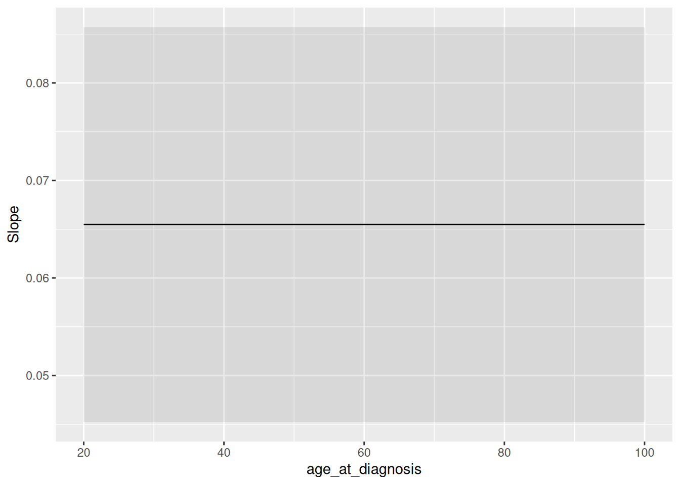
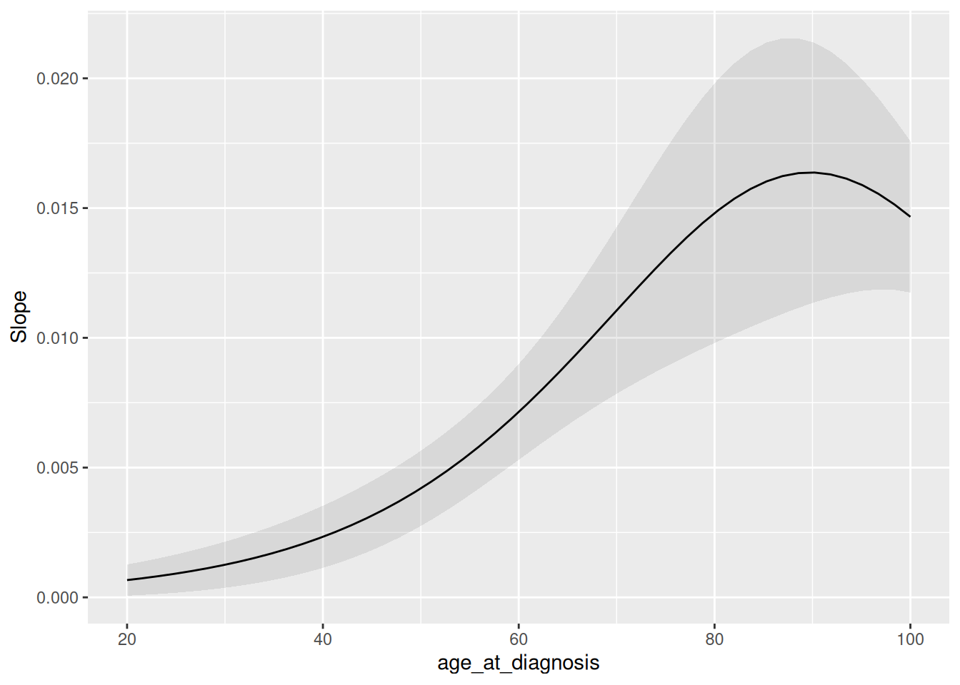
The logistic curve is relatively flat near 0 and 1, and steepest in the middle.
Therefore:
There is not necessarily one single “effect of X” on probability.
plot_slopes(
  th_model,
  condition = "age_at_diagnosis",
  variables = "age_at_diagnosis",
  type = "link"
)
plot_slopes(
  th_model,
  condition = "age_at_diagnosis",
  variables = "age_at_diagnosis",
  type = "response"
)
15.9.4 Thought experiment:
If you’re already likely to die, will adding risk change something?
grid1 = datagrid(
    age_at_diagnosis = 100,
    prior_diabetes = 1,
    thrombectomy = 0,
    model = th_model
)

plot_predictions(
  th_model,
  newdata = grid1,
  variable = "prior_hypertention",
  by = "prior_hypertention"
)

grid2 = datagrid(
    age_at_diagnosis = 70,
    prior_diabetes = 1,
    thrombectomy = 0,
    model = th_model
)

plot_predictions(
  th_model,
  newdata = grid2,
  variable = "prior_hypertention",
  by = "prior_hypertention"
)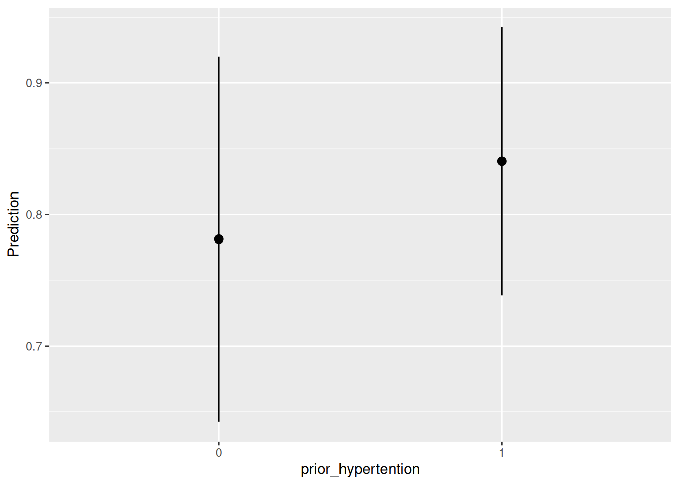
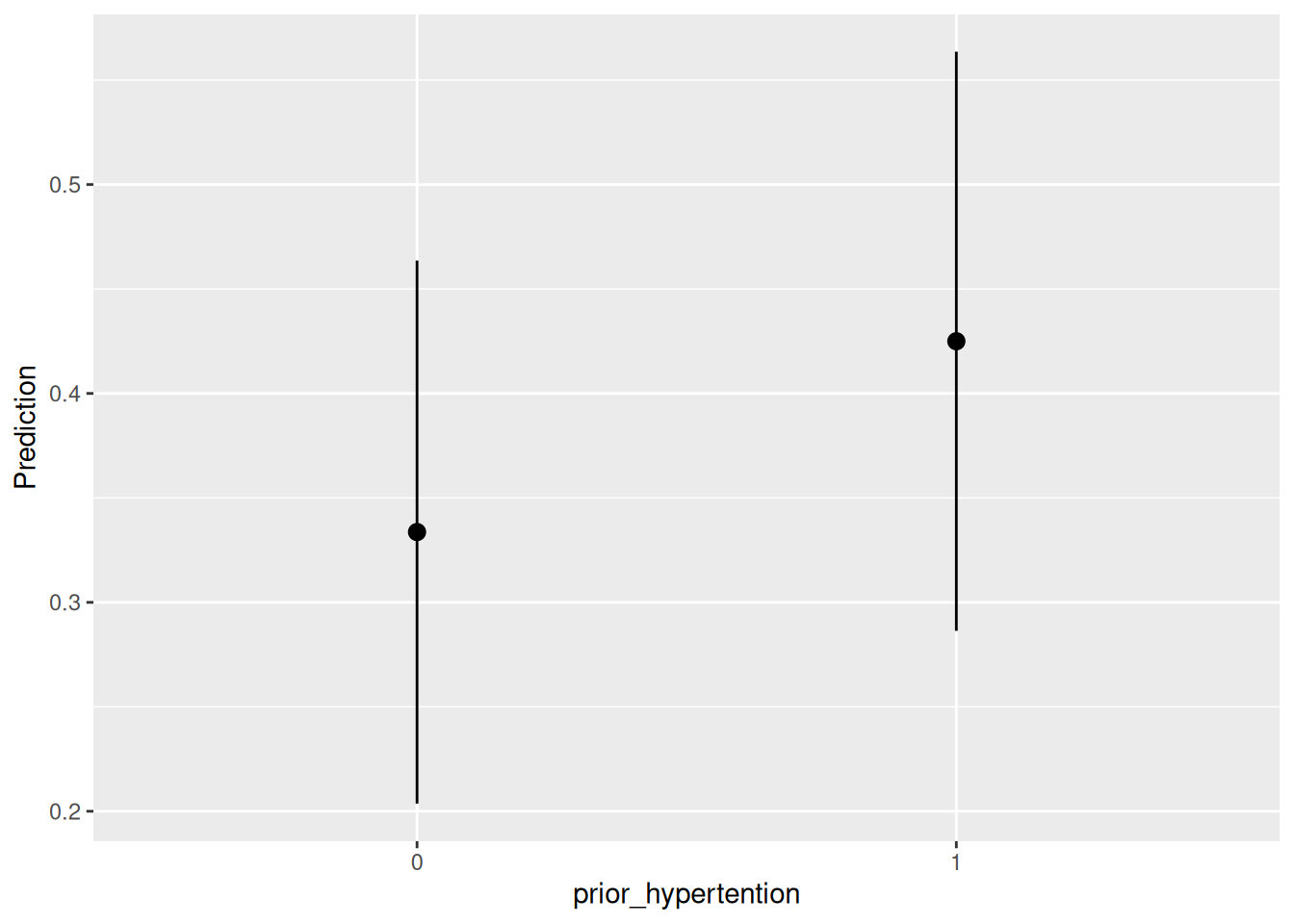
So only a 6% point absolute difference (78.1% to 84.1%) probability for a 100-year-old with diabetes but a 9.1 point absolute difference (33.4% to 42.5%) probability for a 70-year-old with diabetes, both not receiving thrombectomy.
15.10 Step 4: Clear communication — transforming coefficients
Recall Section 13.10 where we learned how to plug in numbers from a fitted regression in order to fit expectations or predictions of specific patients profiles in the dataset.
We will do this again - but this time, we’re fitting a logistic regression
b = coef(th_model)
b
(Intercept) thrombectomy
-6.30743079 2.20414044
prior_diabetes age_at_diagnosis
0.99219918 0.06548817
prior_hypertention sex
0.38930725 0.03936706
thrombectomy:prior_diabetes thrombectomy:age_at_diagnosis
0.49240096 -0.02760921
thrombectomy:prior_hypertention thrombectomy:sex
-0.84966243 0.29304514 linpred_treatment_diabetes_50yo_female = b[1] +
b[2] * 1 + b[3] * 1 + b[4] * 50 + b[5] * 0 +
b[6] * 0 + b[7] * 1 + b[8] * 50 + b[9] * 0 + b[10] * 0
linpred_treatment_diabetes_50yo_female |> unname()[1] -0.7247424| Term | Value | Comment |
|---|---|---|
b[1] |
* 1 |
intercept |
b[2] |
* 1 |
thrombectomy = 1 |
b[3] |
* 1 |
diabetes = 1 |
b[4] |
* 50 |
age = 50 |
b[5] |
* 0 |
hypertension = 0 |
b[6] |
* 0 |
female = 0 |
b[7] |
* 1 |
thrombectomy * diabetes = 1*1 |
b[8] |
* 50 |
thrombectomy * age = 1*50 |
b[9] |
* 0 |
thrombectomy * hypertension = 1*0 |
b[10] |
* 0 |
thrombectomy * sex = 1*0 |
The other will be
linpred_no_treatment_diabetes_40yo_male = b[1] +
    b[2] * 0 + b[3] * 1 + b[4] * 40 + b[5] * 0 +
    b[6] * 1 + b[7] * 0 + b[8] * 0 + b[9] * 0 + b[10] * 0

linpred_no_treatment_diabetes_40yo_male |> unname()
[1] -2.656338| Term | Value | Comment |
|---|---|---|
b[1] |
* 1 |
intercept |
b[2] |
* 0 |
thrombectomy = 0 |
b[3] |
* 1 |
diabetes = 1 |
b[4] |
* 40 |
age = 40 |
b[5] |
* 0 |
hypertension = 0 |
b[6] |
* 1 |
male = 1 |
b[7] |
* 0 |
thrombectomy * diabetes = 0 |
b[8] |
* 0 |
thrombectomy * age = 0*40 |
b[9] |
* 0 |
thrombectomy * hypertension = 0 |
b[10] |
* 0 |
thrombectomy * sex = 0 |
But we’re still in log-odds space. Let’s convert
The letter g represents the standard logistic function
\[ g(x) = \frac{1}{1 + e^{-x}} \]
Applying this function ensures that the linear component inside the parentheses of Equation 5.1 gets rescaled to the interval in order to respect the natural (probability) scale of the binary outcome.
In R, we can make a function to do this for us:
[1] 0.3263495g(linpred_no_treatment_diabetes_40yo_male)[1] 0.06559945# A tibble: 2 × 5
thrombectomy prior_diabetes age_at_diagnosis prior_hypertention sex
<dbl> <dbl> <dbl> <dbl> <dbl>
1 1 1 50 0 0
2 0 1 40 0 1Now, the marginaleffects function predictions() can take care of all this for us:
library(marginaleffects)

predictions(th_model, newdata = grid, type = "link")
 Estimate Std. Error     z Pr(>|z|)    S 2.5 % 97.5 %
   -0.725      0.470 -1.54    0.123  3.0 -1.65  0.196
   -2.656      0.445 -5.97   <0.001 28.7 -3.53 -1.784

Type: link
If we don’t specify type = "link", the default value is type = "response", which has already transformed the log-odds to probability (or log-ratio to count, was the model poisson regression):
predictions(th_model, newdata = grid)
 Estimate Pr(>|z|)    S  2.5 % 97.5 %
   0.3263    0.123  3.0 0.1617  0.549
   0.0656   <0.001 28.7 0.0285  0.144

Type: invlink(link)
15.11 Step 5-7: Model-based transformations
To get the best estimate of our estimand, we need to do some post-hoc transformations to our model coefficients.
Our model is conditional on our sample — we cannot do anything about that. We can, however, do some post-hoc weigh on certain participant profiles, so that our estimate is targeting a specific aspect of the model inference.
Questions that form such discussions can be:
- A particular patient?
- A clinically meaningful scenario?
- The average population?
- Different levels of an interacting variable?
Here, we tackle one scientific question at a time in order to address these questions:
15.11.1 RQ 1: Our sample as reality
“Does the population who got thrombectory have lower probability of death at 1-year follow-up after stroke compared to the population who did not get thrombectomy?”
Here, we’re interested in the sample we have. We’re not asking questions whether these people are representative, biased, or we have any confounds.
The approach we STRONGLY RECOMMEND NOT TO USE is to simply report the coefficients:
th_model |>
    parameters::parameters(exponentiate=TRUE)
# A tibble: 10 × 9
Parameter Coefficient SE CI CI_low CI_high z df_error
<chr> <dbl> <dbl> <dbl> <dbl> <dbl> <dbl> <dbl>
1 (Intercept) 0.00182 1.55e-3 0.95 3.25e-4 9.18e-3 -7.41 Inf
2 thrombecto… 9.06 1.03e+1 0.95 9.82e-1 8.49e+1 1.94 Inf
3 prior_diab… 2.70 7.43e-1 0.95 1.57e+0 4.64e+0 3.60 Inf
4 age_at_dia… 1.07 1.10e-2 0.95 1.05e+0 1.09e+0 6.34 Inf
5 prior_hype… 1.48 2.99e-1 0.95 9.94e-1 2.20e+0 1.92 Inf
6 sex 1.04 2.09e-1 0.95 7.02e-1 1.54e+0 0.196 Inf
7 thrombecto… 1.64 7.60e-1 0.95 6.57e-1 4.08e+0 1.06 Inf
8 thrombecto… 0.973 1.39e-2 0.95 9.46e-1 1.00e+0 -1.93 Inf
9 thrombecto… 0.428 1.41e-1 0.95 2.23e-1 8.12e-1 -2.58 Inf
10 thrombecto… 1.34 4.32e-1 0.95 7.14e-1 2.53e+0 0.908 Inf
# ℹ 1 more variable: p <dbl>Here, the odds ratio is 2.20 …
when all interacting variables are at their reference/zero values.
In particular, the interpretation depends on how age is coded/centered and on the reference categories for diabetes, hypertension, and sex.
But how intuitive is that? 👀
Instead, lets make predictions on the outcome scale of probabilities using marginaleffects.
If we don’t supply a newdata grid, the predictions() function will take all participants in our sample and compute predictions for them, one by one:
p = predictions(th_model)
p
 Estimate Pr(>|z|)    S  2.5 % 97.5 %
   0.2677   <0.001 28.9 0.2083  0.337
   0.0706   <0.001 40.2 0.0361  0.133
   0.3220   <0.001 19.9 0.2606  0.390
   0.1979   <0.001 36.8 0.1417  0.269
   0.1275   <0.001 40.1 0.0794  0.198
--- 1013 rows omitted. See ?print.marginaleffects ---
   0.4588    0.683  0.6 0.2776  0.652
   0.6696    0.102  3.3 0.4651  0.825
   0.3413    0.137  2.9 0.1788  0.552
   0.4494    0.617  0.7 0.2694  0.644
   0.6611    0.118  3.1 0.4575  0.819
Type: invlink(link)
You can see that the row length is the same as the original dataset:
A table with 1023 rows is not super intuitive and nice to make inference from. Why can we do about that?
We could either
- Make a plot to illustrate it all visually, or
- take the average of all these predictions
Keeping all information
Let’s start by the first approach and visualize all information:
library(patchwork)

p = predictions(th_model)

# Histogram
p1 = ggplot(p) +
  geom_histogram(aes(estimate, fill = factor(thrombectomy))) +
  labs(x = "Pr(outcome = 1)", y = "Count", fill = "thrombectomy") +
  scale_fill_grey()

# Empirical Cumulative Distribution Function
p2 = ggplot(p) +
  stat_ecdf(aes(estimate, colour = factor(thrombectomy))) +
  labs(x = "Pr(outcome = 1)",
       y = "Cumulative Probability",
       colour = "thrombectomy") +
  scale_colour_grey()

# Combined plots
p1 + p2
`stat_bin()` using `bins = 30`. Pick better value `binwidth`.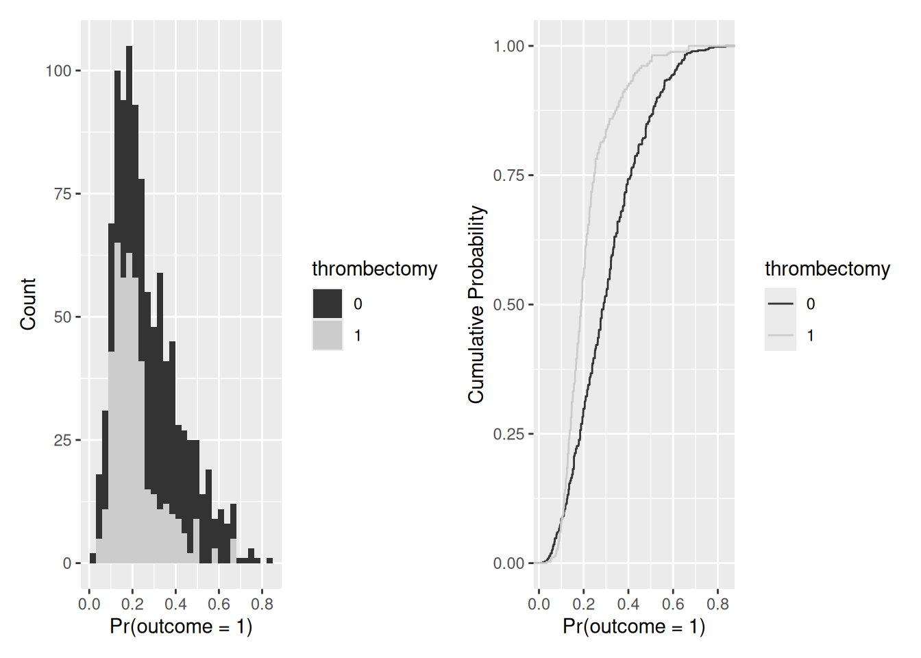
The plot to the left shows the histogram. I suddenly becomes clear that fewer patients received thrombectomy than patients who did not.
Indeed, that is correct:
table(thrombectomy$thrombectomy)
  0   1
583 440
about 0.4301075 received thrombectomy.
From the right plot, we can see the cumulative density plot. Here, it seems that overall…
Marginalizing over the predictions
We can compute the average for them by using avg_predictions()
avg_predictions(th_model)
 Estimate Std. Error    z Pr(>|z|)     S 2.5 % 97.5 %
    0.267      0.013 20.5   <0.001 307.1 0.241  0.292

Type: response
So the average probability of death at the 1-year follow-up is 26.7%.
This is a reasonable estimate for answering the question
“how many Danes die at 1-year follow-up after stroke?”
However, as we now know that the groups are unbalanced, this is not a good estimate for the treatment effect! And it doesn’t have the granularity to address more nuanced questions of sub-population level.
Finally, to compute the average for the patients receiving thrombectomy and those who did not, we can group the average for these conditions
avg_predictions(th_model, by="thrombectomy")
 thrombectomy Estimate Std. Error    z Pr(>|z|)     S 2.5 % 97.5 %
            0    0.307     0.0179 17.1   <0.001 216.0 0.272  0.342
            1    0.214     0.0188 11.4   <0.001  96.8 0.177  0.251

Type: response
Based on the data we have, patients that are offered and successfully manage to receive thrombectomy have a 30.7% and 21.4% chance of death measured at 1-year follow-up.
This is the final estimate for our question:
“Do Danish patients who receive thrombectomy have better probability of survival at 1-year follow-up after stroke, compared to patients not receiving thrombectomy?”
However, a better estimate might be the risk difference or the risk ratio.
\[ RD = 0.214 - 0.307 = -9.3 \] or a 9.3% points lower predicted risk of death on the absolute scale.
\[ RR = \frac{0.214}{0.307} = 0.697 \] or a 30% lower predicted risk of death on the relative scale.
So we conclude that:
The model-estimated 1-year mortality was 30.7% in the absence of thrombectomy and 21.4% under thrombectomy, corresponding to an un-adjusted absolute risk difference of −9.3 percentage points
15.11.2 RQ 2: Treatment effect of older adults conditional on diabetes status
“What is the effect of thrombectory in older adults with diabetes, compared to older adults without diabetes?”
Here, we’re interested specifically in a sub-population. So now, we need to consider multiple variables (diabetes and thrombectory) and the proportions who have this profile in our sample.
# A tibble: 22 × 6
   rowid prior_hypertention   sex prior_diabetes thrombectomy
   <int>              <int> <int>          <dbl>        <dbl>
 1     1                  1     1              1            0
 2     2                  1     1              1            0
 3     3                  1     1              1            0
 4     4                  1     1              1            0
 5     5                  1     1              1            0
 6     6                  1     1              1            0
 7     7                  1     1              1            0
 8     8                  1     1              1            0
 9     9                  1     1              1            0
10    10                  1     1              1            0
# ℹ 12 more rows
# ℹ 1 more variable: age_at_diagnosis <int>
p = predictions(
th_model,
newdata = datagrid(
prior_diabetes = 1,
thrombectomy = c(0, 1),
age_at_diagnosis=c(80:90)
)
)
p
 prior_diabetes thrombectomy age_at_diagnosis Estimate Pr(>|z|)   S
              1            0               80    0.587  0.22571 2.1
              1            0               81    0.603  0.15388 2.7
              1            0               82    0.619  0.10197 3.3
              1            0               83    0.634  0.06589 3.9
              1            0               84    0.649  0.04165 4.6
              1            0               85    0.664  0.02586 5.3
              1            0               86    0.678  0.01582 6.0
              1            0               87    0.692  0.00958 6.7
              1            0               88    0.706  0.00576 7.4
              1            0               89    0.719  0.00345 8.2
              1            0               90    0.733  0.00206 8.9
              1            1               80    0.570  0.42785 1.2
              1            1               81    0.580  0.37336 1.4
              1            1               82    0.589  0.32461 1.6
              1            1               83    0.598  0.28134 1.8
              1            1               84    0.607  0.24322 2.0
              1            1               85    0.616  0.20986 2.3
              1            1               86    0.625  0.18082 2.5
              1            1               87    0.634  0.15567 2.7
              1            1               88    0.643  0.13397 2.9
              1            1               89    0.651  0.11531 3.1
              1            1               90    0.660  0.09930 3.3
 2.5 % 97.5 %
 0.446  0.716
 0.461  0.730
 0.476  0.743
 0.491  0.757
 0.506  0.770
 0.520  0.782
 0.535  0.794
 0.549  0.806
 0.563  0.817
 0.577  0.828
 0.591  0.839
 0.397  0.728
 0.405  0.737
 0.412  0.745
 0.419  0.754
 0.427  0.762
 0.434  0.771
 0.441  0.779
 0.448  0.787
 0.455  0.795
 0.462  0.802
 0.469  0.810

Type: invlink(link)predictions(
th_model,
newdata = datagrid(
age_at_diagnosis = 80,
prior_diabetes = unique,
thrombectomy = max
)
)
 age_at_diagnosis prior_diabetes thrombectomy Estimate Pr(>|z|)    S
               80              0            1    0.231   <0.001 22.2
               80              1            1    0.570    0.428  1.2
 2.5 % 97.5 %
 0.161  0.321
 0.397  0.728

Type: invlink(link)predictions(
th_model,
newdata = datagrid(
age_at_diagnosis=c(80:90),
prior_diabetes = unique,
thrombectomy = max)
)
 age_at_diagnosis prior_diabetes thrombectomy Estimate Pr(>|z|)    S
               80              0            1    0.231  < 0.001 22.2
               80              1            1    0.570  0.42785  1.2
               81              0            1    0.238  < 0.001 20.5
               81              1            1    0.580  0.37336  1.4
               82              0            1    0.245  < 0.001 18.8
               82              1            1    0.589  0.32461  1.6
               83              0            1    0.252  < 0.001 17.2
               83              1            1    0.598  0.28134  1.8
               84              0            1    0.259  < 0.001 15.7
               84              1            1    0.607  0.24322  2.0
               85              0            1    0.267  < 0.001 14.2
               85              1            1    0.616  0.20986  2.3
               86              0            1    0.274  < 0.001 12.9
               86              1            1    0.625  0.18082  2.5
               87              0            1    0.282  < 0.001 11.6
               87              1            1    0.634  0.15567  2.7
               88              0            1    0.289  < 0.001 10.5
               88              1            1    0.643  0.13397  2.9
               89              0            1    0.297  0.00148  9.4
               89              1            1    0.651  0.11531  3.1
               90              0            1    0.305  0.00293  8.4
               90              1            1    0.660  0.09930  3.3
 2.5 % 97.5 %
 0.161  0.321
 0.397  0.728
 0.165  0.331
 0.405  0.737
 0.169  0.341
 0.412  0.745
 0.174  0.351
 0.419  0.754
 0.178  0.362
 0.427  0.762
 0.182  0.373
 0.434  0.771
 0.186  0.384
 0.441  0.779
 0.191  0.395
 0.448  0.787
 0.195  0.407
 0.455  0.795
 0.199  0.418
 0.462  0.802
 0.204  0.430
 0.469  0.810

Type: invlink(link)avg_predictions(
th_model,
newdata = datagrid(
age_at_diagnosis=c(80:90),
prior_diabetes = unique,
thrombectomy = max)
)
 Estimate Std. Error    z Pr(>|z|)    S 2.5 % 97.5 %
    0.442     0.0577 7.65   <0.001 45.6 0.328  0.555

Type: response
grid_oi <- datagrid(
age_at_diagnosis=c(80:90),
prior_diabetes = unique,
thrombectomy = unique,
model = th_model
)
p1 = plot_predictions(th_model, newdata = grid_oi, by = "thrombectomy")
p2 = plot_predictions(th_model, newdata = grid_oi, by = c("thrombectomy", "prior_diabetes"))
p1 + p2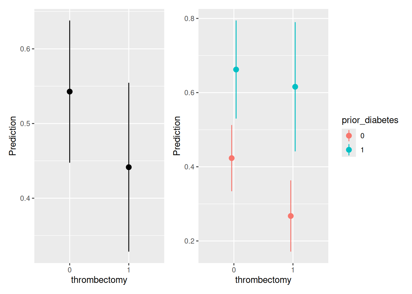
It becomes clear that the effect of thrombectomy on 1-year follow-up mortality is negated substantially by the co-occurrence of diabetes in old age.
The effect is substantial for non-diabetic old patient.
avg_predictions(
    th_model,
    by = c("thrombectomy", "prior_diabetes"),
    newdata = datagrid(
        age_at_diagnosis=c(80:90),
        prior_diabetes = unique,
        thrombectomy = unique
    )
)
 thrombectomy prior_diabetes Estimate Std. Error    z Pr(>|z|)    S
            0              0    0.423     0.0455 9.30   <0.001 65.9
            0              1    0.662     0.0674 9.82   <0.001 73.2
            1              0    0.267     0.0490 5.46   <0.001 24.3
            1              1    0.616     0.0889 6.93   <0.001 37.8
 2.5 % 97.5 %
 0.334  0.513
 0.530  0.794
 0.171  0.363
 0.442  0.790

Type: response
from 42.3% probability of death without treatment to 26.7% for non-diabetic.
from 66.2% probability of death without treatment to 61.6% for non-diabetic.
So our estimates are
15.11.3 RQ:3 “The average person”
What is effect of the average person profile in the sample?
Until now, we have considered our observations as meaningful populations that we want to investigate. However, if we’re interested in thrombectomy as an experimental procedure for any possible candidate patient, we have until now treated the groups unfairly.
But realistictly, people who gets hit by a stroke and need thrombectomy are not “any one”. These people are already a specific sub-population of Danish people. Therefore, a perfectly balanced age group, 50% diabetes etc. is extremely unrealistic and not representative of the Danish population.
First of all, males are nearly 48% propensity of receiving thrombectory or not, while it’s only 38% of females.
xtabs(~ thrombectomy + sex, data=thrombectomy) sex
thrombectomy 0 1
0 308 275
1 190 250We have many more males in the treatment group and
xtabs(~ thrombectomy + prior_diabetes, data=thrombectomy) prior_diabetes
thrombectomy 0 1
0 512 71
1 400 40We don’t have equal amount of patients with diabetes in the treatment group.
About 10-15% of our sample have diabetes (while the Danish prevalence is 6,4%). A balanced design would have 50% in each group (although this is unrealistic in reality).
We might be interested in covering some representative and balanced parts of the population.
age_mean <- mean(thrombectomy$age_at_diagnosis)
age_sd <- sd(thrombectomy$age_at_diagnosis)

grid_oi <- datagrid(
    model = th_model,
    prior_diabetes = unique,
    prior_hypertention = unique,
    sex = unique,
    thrombectomy = unique,
    age_at_diagnosis = c(age_mean-age_sd, age_mean, age_mean+age_sd)
    )

predictions(
    th_model,
    by = "thrombectomy",
    newdata = grid_oi
)
 thrombectomy Estimate Std. Error     z Pr(>|z|)    S 2.5 % 97.5 %
            0    0.334     0.0296 11.29   <0.001 95.8 0.276  0.392
            1    0.365     0.0432  8.45   <0.001 54.9 0.280  0.450

Type: response
This grid is perfectly balanced at our representative selected age: 60, 73, and 86 years old. We have the same amount of diabetes, hypertension, males, and thrombectomy. This is indeed a completely made-up example. But so is “the average person”! 👀
Warning“The average person” doesn’t exist!
In some samples, “the average person” doesn’t exist. I mean this literally 😅
Consider the case where we have a bimodal distribution — either people love or hate coriander/cilantro. There is noone who is “meh”. So computing the average person would be the awkward average of “meh”, while in reality, people are either excited or disgusted.
Imagine a scenario where a patient either benefits a lot or not at all from a treatment. The “average person” would then get “some moderate effect” — but that would be completely against the clinical reality experienced by the clinicians! 👀
p1 = plot_predictions(
    th_model,
    newdata = grid_oi,
    condition = "age_at_diagnosis"
)
p2 = plot_predictions(
    th_model,
    newdata = grid_oi,
    condition = c("age_at_diagnosis", "thrombectomy")
)
p3 = plot_predictions(
    th_model,
    newdata = grid_oi,
    condition = c("age_at_diagnosis", "thrombectomy", "prior_diabetes")
)
(p1 + p2) / p3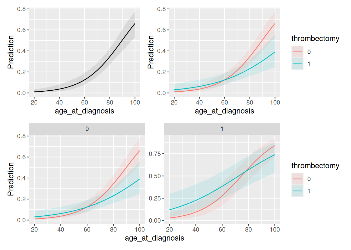
15.11.4 RQ 4: “What if” 🤔
The research questions was:
What would be the average probability of death, had all participants received thrombectomy, compared to not receiving it?
Finally, we might be interested in the imaginary scenario: what had happened, given all patients received both the treatment and no treatment, and which would have resulted in the best probability of being alive at the 1-year follow-up?
We can actually ask this question too:
p = predictions(th_model, variables = list(thrombectomy = 0:1))
nrow(p)
[1] 2046Notice how our dataset just doubled its rows. This is no coicidence!
In fact, we now have all observed participants with the “counterfactual” reality that they both got thrombectomy and not. It is called counterfactual because is its “counter to the fact”. The fact was that each patient either did or did not revieve the thrombectomy. Counter to this fact, we’re interested in the imaginary scenario that they got both!
These predictions are interesting, because they give us a first look at the kinds of counterfactual (potentially causal) queries.
We can ask:
For each individual in the
Syntheric DanStrokemedisr sample, what is the predicted probability of death in the counterfactual world where they receive thrombectory, and where they do not?
Let’s marginalize over all participant profiles and get the average probability of death, had everyone in the sample been in both scenarios of the treatment/no-treatment.
avg_predictions(th_model, variables = list(thrombectomy = 0:1))
 thrombectomy Estimate Std. Error    z Pr(>|z|)     S 2.5 % 97.5 %
            0    0.271     0.0168 16.1   <0.001 191.8 0.238  0.304
            1    0.239     0.0212 11.3   <0.001  95.6 0.198  0.281

Type: response
Notice how different the probabilities are now. Remember that the dataset is not balanced — but rather symmetric between the two groups now. The sample is still biased by propensity for having diabetes, hypertension etc. But the treatment groups share all these biases now.
plot_predictions(
    th_model,
    newdata=datagrid(
        thrombectomy = c(0,1),
        grid_type="counterfactual"
    ),
    by="thrombectomy"
)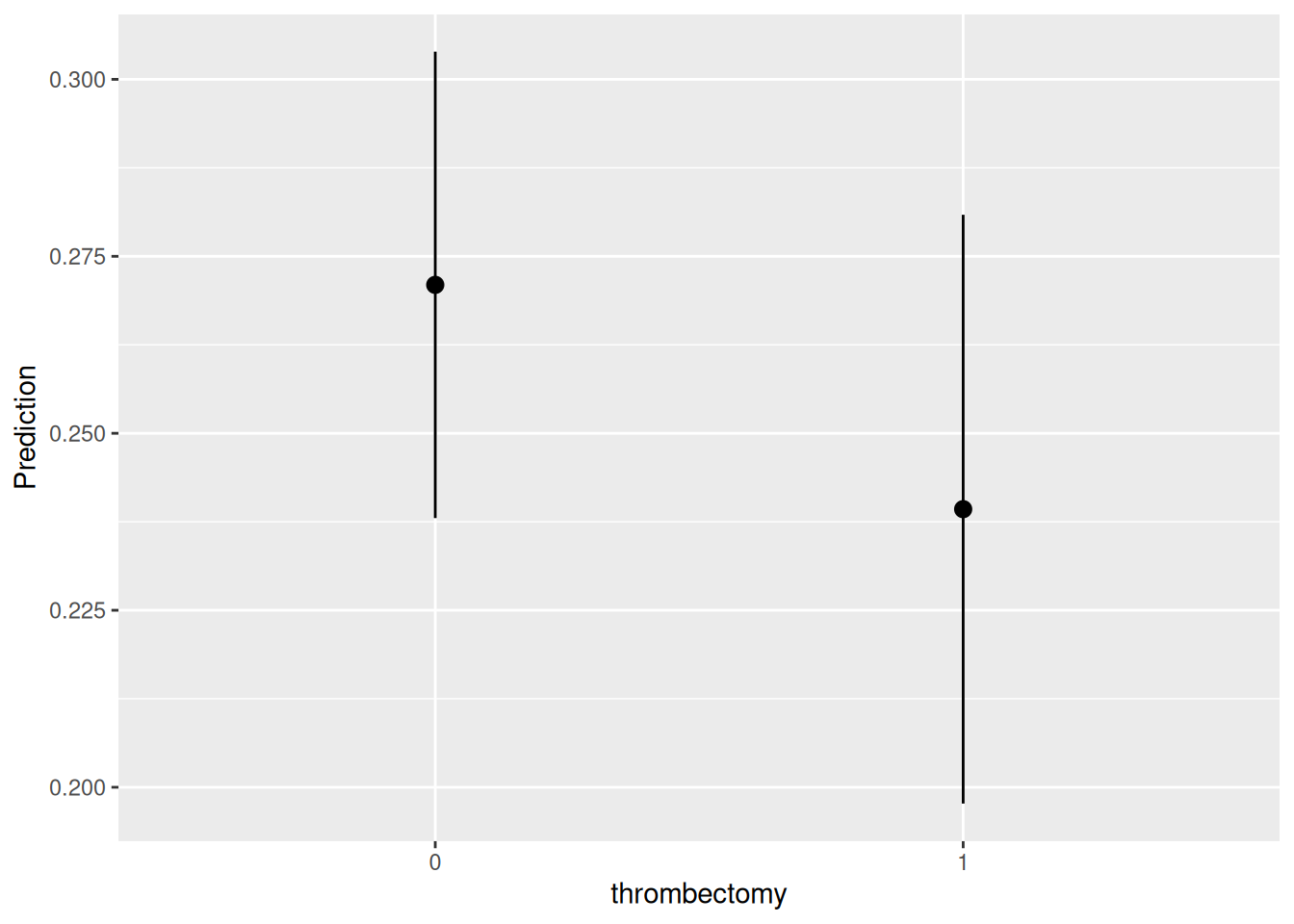
This is the best estimate we have until now for the question:
“Would Danish stroke patients have lower probability of death at 1-year follow-up after stroke if everyone had received thrombectomy compared to not receiving it?”
However, a better estimate might be the risk difference or the risk ratio.
avg_comparisons(
    th_model,
    variables = "thrombectomy"
    )
 Estimate Std. Error     z Pr(>|z|)   S   2.5 % 97.5 %
  -0.0317     0.0271 -1.17    0.242 2.0 -0.0847 0.0214

Term: thrombectomy
Type: response
Comparison: 1 - 0
So a risk difference of -0.0317, favoring thrombectomy (negative probability subtracting the probability of death for patients revieving thrombectomy - patients not revieving thrombectomy).
The comparisons() function above computed the predicted probability of mortality (death_1year_followup == 1) for each observed row of the data in two counterfactual cases: when thrombectomy == 1, and when thrombectomy == 0. Then, it computed the differences between these two sets of predictions. Finally, it computed the population-average of risk differences.
Instead of risk differences, we could compute population-averaged (marginal) adjusted risk ratios:
avg_comparisons(
    th_model,
    variables="thrombectomy",
    comparison = "lnratioavg", # Calculates adjusted Risk Ratio
    transform = exp # then exponentiates
    )
 Estimate Pr(>|z|)   S 2.5 % 97.5 %
    0.883    0.251 2.0 0.714   1.09

Term: thrombectomy
Type: response
Comparison: ln(mean(1) / mean(0))
Which gives the estimate of a 0.883 adjusted risk ratio after revieving thrombectomy.
So we conclude that:
The model-estimated 1-year mortality was 27.1% in the absence of thrombectomy and 23.9% under thrombectomy, corresponding to an adjusted risk ratio of 0.883.
15.12 Summary
This session covered going from estimand to estimate.
To communicate clearly about results, we need to apply transformations to our model coefficients. Predictions can be computed on different scales, depending on the type of statistical model. The quantity we use should be intuitive and relevant for clinical practice (going from OR to model-based probabilities)
Analysts can make predictions for different combinations of predictor values, or grids: empirical, interesting, representative, balanced, or counterfactual. The grid depends on the research estimatand.
To simplify the presentation of results, it often makes sense to report average predictions (i.e. marginalizing over all predictions).