While causal models are great for knowing how effective a thing is, sometimes you just want to know how likely this is to happen.
For example, suppose you’re into gambling and want to bet money on horse rides at Aalborg Travbane. You don’t need info on why a particylar jokey and horse wins — you’ll be happy just knowing whether it wins or not. The great thing about prediction models is that it will take any horse and provide a prediction. Thus, prediction models are capable of making individual judgements.
But consider the counter example. You are told that your dog is sick and will likely die. This information is worthless without knowing what to do about it. You want an intervention — a trick to counteract the sickness. This requires causal information. Often, the veterinarian will not know exactly what your dog needs, but they will know that any dog will get sick from eating chocolate. Indeed, some unique dogs might tolerate it better, but the negative effect is causal on a population level.
Most scientific fields bennefit from both approaches. Take the weather, for example. The majority of people don’t care why it will rain or why the temperature drops 10 degrees over night. But it is expremely useful information the industry (formers, sailors, outdoor events, public transportation). And most people want to know the weather in their specific part of the world. But in the face of climate change, we also need to know why the earth is experiencing global warming. Just knowing that the earth will be 1.2 degrees warmer in 10 years will not help us keep the temperature lower or prevent the disaster.
Read about this PhD-project at AAU: https://www.cs.aau.dk/kunstig-intelligens-kan-forudsige-hvor-laenge-du-skal-vaere-indlagt-n89354?utm
Discuss:
How are variable selection and confounding treated in prediction models?
What decision does the prediction help with?
Could a variable be very useful for predicting length of stay without causing a longer stay?
Would you trust the model if it made very accurate predictions but you didn’t understand why it worked?
What would be different if the hospital wanted to know what intervention would shorten the patient’s stay?
Prediction models cannot inform intervention. Only risk assessment and potential willingness to act — but what to act on?
The ad_validation_logistic data are particularly convenient because they already contain observed classes and out-of-sample predicted probabilities from a logistic regression model.
16.5.1 Dataset context:
The dataset was made based on the following logistic regression classifier:
# Logistic regressionmodel<-glm(impairment~age+male+tau+p_tau+Ab_42+Genotype, data =train, family =binomial)
So
\[
impairment_i \sim age + male + tau + p\_tau + Ab\_42 + genotype
\] where:
age: Normalized unit
male: Reported sex was male
tau: Tau protein stabilizes microtubules in axons. They can form insoluble neurofibrillary tangles when floating around freely. Here, the concentration was measured in the cerebrospinal fluid via lumbar puncture.
p_tau: Phosphorylated tau neurofibrillary tangles in the cerebrospinal fluid. Here, the concentration was measured in the cerebrospinal fluid via lumbar puncture.
Ab_42: Amyloid beta 42 (Aβ42) is a 42-amino-acid peptide derived from the amyloid precursor protein that forms the plaques found in the brains of people with Alzheimer’s disease.
genotype: The APOE allele pair. Can be E2E2, E2E3, E3E3, E3E4, E2E4, or E4E4. .
We want to predict patients with cognitive impairment defined by a gold-standard neurophyschological test (such as the Wechsler’s Adult Intelligence Score).
# A tibble: 167 × 7
   diagnosis   age  male   tau p_tau Ab_42 Genotype
   <fct>     <dbl> <int> <dbl> <dbl> <dbl> <fct>
 1 control   0.988     0  6.30  4.35 12.0  E2E2
 2 control   0.987     1  6.27  4.40 12.3  E2E3
 3 control   0.987     0  6.62  4.52 11.0  E2E2
 4 control   0.985     1  5.74  3.75 14.3  E3E4
 5 control   0.984     0  4.98  3.46 13.7  E2E2
 6 impaired  0.986     0  6.16  4.43  9.76 E2E3
 7 impaired  0.984     1  5.06  3.29 11.3  E2E2
 8 control   0.988     0  6.25  4.52 12.2  E2E2
 9 impaired  0.986     1  5.99  4.13 11.9  E2E2
10 control   0.988     0  4.77  3.33 11.3  E2E2
# ℹ 157 more rows
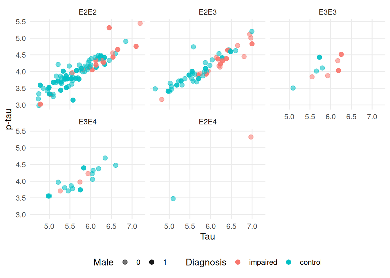
p1<-ggplot(test, aes(tau, p_tau, colour =diagnosis))+geom_point(aes(alpha =factor(male)), size =2.4, position =position_jitter(width =0.03, height =0.03))+facet_wrap(~Genotype)+scale_alpha_manual( values =c(`0` =0.55, `1` =0.9), name ="Male")+labs( x ="Tau", y ="p-tau", colour ="Diagnosis")+theme_minimal(base_size =12)+theme( panel.grid.minor =element_blank(), legend.position ="bottom")p1
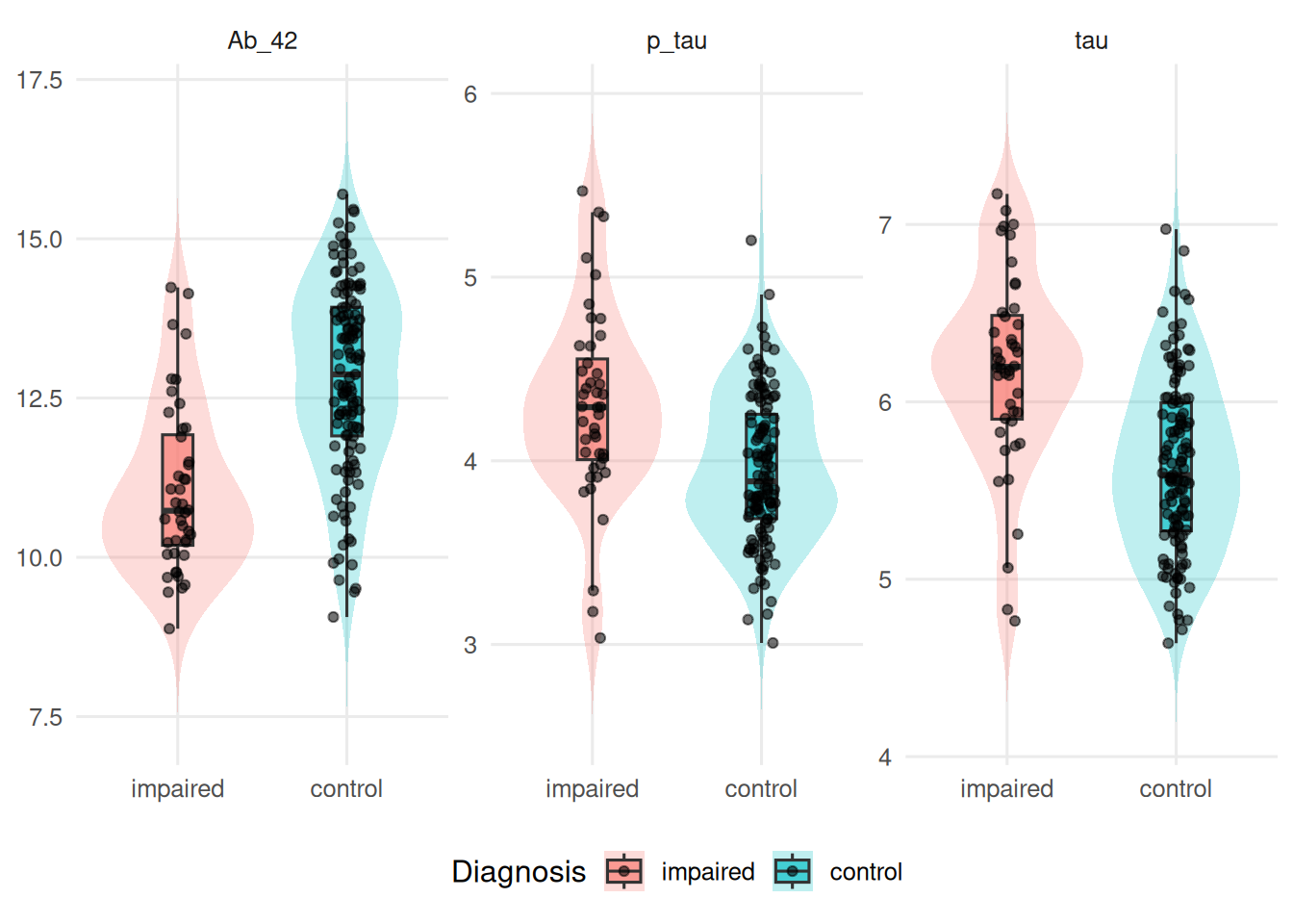
biomarkers<-test|>pivot_longer( cols =c(tau, p_tau, Ab_42), names_to ="biomarker", values_to ="value")p2<-ggplot(biomarkers,aes(diagnosis, value, fill =diagnosis))+geom_violin( alpha =0.25, colour =NA, trim =FALSE)+geom_boxplot( width =0.18, outlier.shape =NA, alpha =0.65)+geom_jitter( width =0.08, height =0, size =1.4, alpha =0.55)+facet_wrap(~biomarker, scales ="free_y")+labs( x =NULL, y =NULL, fill ="Diagnosis")+theme_minimal(base_size =12)+theme( panel.grid.minor =element_blank(), legend.position ="bottom")p2
16.6 Our model to validate:
Step
Specific issues
AlzheimerDisease model
1. Problem definition and data inspection
Aim: predictors or predictions? Selection, predictor definitions, and completeness, endpoint definition
Aim is to determine whether demographic, CSF biomarker, and genetic predictors can be used to predict Alzheimer’s disease/cognitive impairment and to provide individualized predicted probabilities. Data are derived from the AlzheimerDisease dataset based on a clinical study of CSF biomarkers for Alzheimer’s disease. The outcome is diagnosis, with levels impaired and control. The original observations were split by alternating rows, with even-numbered observations used for model training and odd-numbered observations used for validation.
Continuous predictors include normalized age, CSF total tau, phosphorylated tau (p_tau), and amyloid beta 42 (Ab_42). Sex is coded as the binary indicator male. APOE genotype is treated as a categorical predictor with six possible allele-pair categories: E2E2, E2E3, E3E3, E3E4, E2E4, and E4E4.
3. Model specification
Selection of main effects? Assessment of assumptions?
Logistic regression model specified as diagnosis ~ age + male + tau + p_tau + Ab_42 + Genotype. The model includes the specified main effects. No interaction terms or nonlinear transformations are described in the supplied model specification.
4. Model estimation
Shrinkage included?
The logistic regression model was fitted to the even-numbered training observations. No shrinkage or penalization is described in the supplied model specification.
5. Model performance
Appropriate measures used?
Predicted probabilities were generated for the odd-numbered validation observations, including probabilities for the impaired and control classes. Model performance can be assessed using discrimination and calibration; the supplied dataset specifically contains predicted probabilities and observed diagnoses, but does not specify particular performance measures.
6. Model validation
Internal validation including model specification and estimation?
Hold-out validation using the odd-numbered observations. The model was fitted exclusively to the even-numbered training observations and evaluated on the odd-numbered validation observations. This provides validation on observations not used to fit the model.
7. Model presentation
Format appropriate for audience
The validation dataset provides predicted probabilities for both impaired and control diagnoses alongside the observed diagnosis. This format is suitable for evaluating and presenting individual predicted risks, although the underlying logistic regression formula would be needed to reproduce individual predictions.
16.7 Workflow
Table 2. Overview of four measures (ABCD) for model performance
Aspect
Measure
Visualization
Characteristics
Calibration
A: Calibration-in-the-large (α)
Calibration plot
Intercept in the calibration plot; compares the mean observed outcome with the mean predicted probability.
Calibration
B: Calibration slope (β)
Calibration plot
Regression slope in the calibration plot; related to the amount of shrinkage required for the regression coefficients.
Discrimination
C: C-statistic
ROC curve
Interpreted as the probability that the model assigns a higher predicted probability to a randomly selected subject with the endpoint than to a randomly selected subject without the endpoint.
Clinical usefulness
D: Decision-curve analysis (Net Benefit)
Decision curve
Net true-positive classification rate achieved by using the model across a range of decision thresholds.
Figure 16.1
16.8 Evaluating a Prediction Model
A prediction model can be evaluated from two things:
what actually happened;
and what the model predicted.
Here we use predictions from a logistic regression model. The model has already been trained, so we do not fit a model. We simply evaluate its predictions.
We can make a confusion matrix — a table that shows how many observations were classified correctly and how many were assigned to the wrong class.
conf_mat(predictions, truth =Class, estimate =.pred_class)
          Truth
Prediction impaired control
  impaired       25      14
  control        19     109
A confusion matrix is useful because it lets us see what kinds of mistakes the model is making, rather than giving us just one summary number.
We spot an interesting pattern:
There are many more control participants than cognitively impaired participants.
labeling the cognitive impairment was not a success — only 25 out of 44 were labeled correctly!
labeling the control participants much better — 109 out of 123 were labeled correctly!
We can quickly calculate that 0.8861789% of the controls were labeled correctly while only 0.5681818% of the cognitively impaired were labeled correctly.
This seems like a reasonable way to evaluate the model. But there is a problem: these percentages answer a slightly different question for each class, and they can be strongly affected by how common each class is.
In particular, there are many more controls than cognitively impaired participants. A model can therefore appear to perform well simply by being good at predicting the more common class.
So rather than looking only at the percentage of observations classified correctly, we can use metrics that explicitly describe different types of classification errors.
16.10.1 Accuracy
Accuracy answers a simple question:
How often does the model get the class right?
Accuracy is the proportion of all observations that were classified correctly:
$$ Accuracy =
$$
Here, TP means true positives, TN means true negatives, FP means false positives, and FN means false negatives.
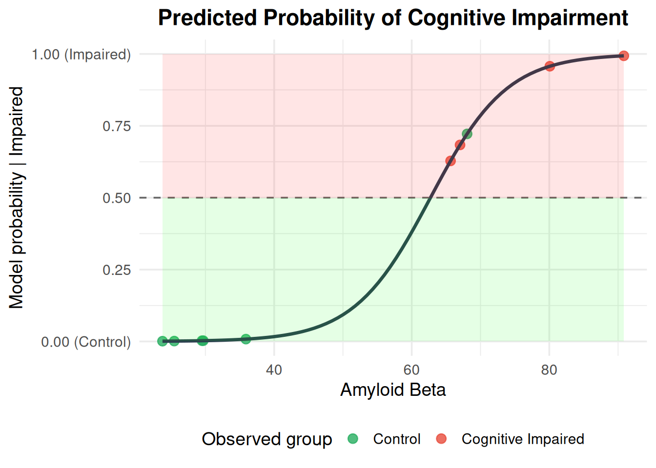
To calculate accuracy, we first turn probabilities into classes. Here we use 0.5 as the threshold: if the predicted probability of impairment is at least 0.5, we classify the participant as impaired; otherwise, we classify them as a control.
The accuracy was 0.802. This means that about 80.2% of all participants were classified correctly.
Accuracy is easy to understand, but it has an important limitation: it does not tell us which class the model gets wrong. It can also be misleading when the classes are unbalanced.
For example, imagine that 95% of participants were controls. A model that always predicted “control” would have 95% accuracy, despite completely failing to identify anyone with cognitive impairment.
This is why it is useful to look separately at the model’s performance for the different classes.
16.10.2 Specificity
Specificity asks:
Among people who are not “impaired”, how many does the model correctly identify?
Specificity measures how well the model identifies the negative class — here, the control participants.
In other words, specificity is the proportion of actual controls that the model correctly labels as controls.
The specificity was 0.886. This means that 88.6% of the participants who were actually controls were correctly identified as controls.
A highly specific model produces few false positives: it rarely labels a control participant as cognitively impaired.
Specificity is therefore particularly useful when false positives are costly or problematic. For example, in a screening context, a false positive might lead to unnecessary further testing or concern.
16.10.3 Sensitivity
Sensitivity asks:
Among people who are “impaired”, how many does the model correctly identify?
Sensitivity measures how well the model identifies the positive class — here, cognitively impaired participants.
\[
Specificity = \frac{TN}{TN + FP}
\]
In other words, sensitivity is the proportion of participants who are actually impaired that the model correctly identifies as impaired.
The sensitivity was 0.568. This means that 56.8% of the participants who were actually cognitively impaired were correctly identified by the model.
A highly sensitive model produces few false negatives: it rarely misses a participant who is actually impaired.
This distinction between sensitivity and specificity is important. A model can have high specificity while having relatively low sensitivity, as we see here. Our model is quite good at recognizing controls, but it misses a substantial proportion of participants with cognitive impairment.
16.10.4 Discussion task: Setting a proability threshold
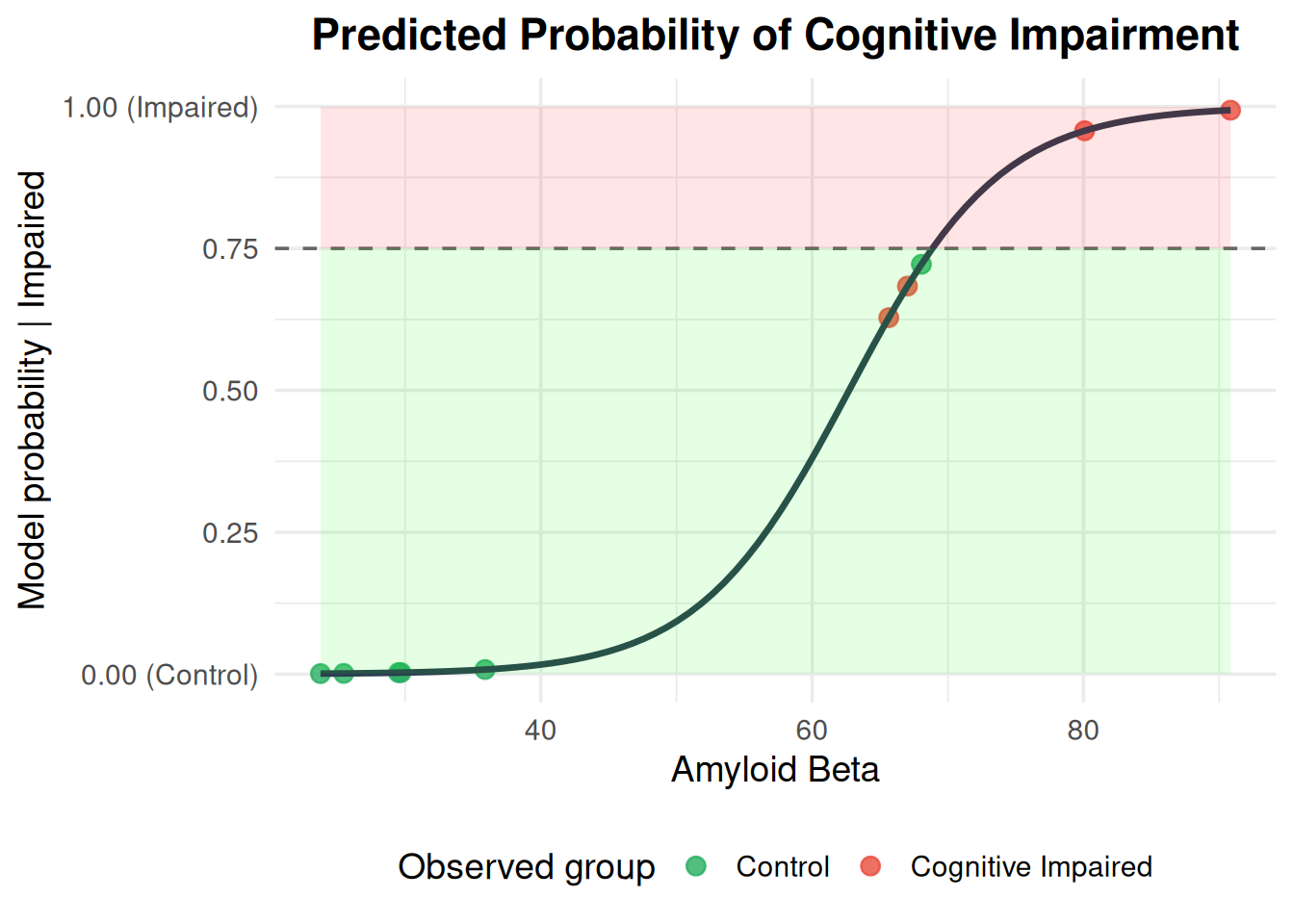
Sensitivity and specificity depend on the chosen probability threshold. We used 0.5 above, but there is nothing inherently special about 0.5.
Changing the threshold changes the balance between false positives and false negatives. A lower threshold makes the model more willing to classify someone as impaired. This will generally increase sensitivity, because fewer impaired participants are missed, but it can also decrease specificity, because more controls may be incorrectly labeled as impaired.
Conversely, a higher threshold makes the model more conservative about calling someone impaired. This can increase specificity but may reduce sensitivity.
In a clinical application, the useful threshold should therefore be chosen based on the consequences of the two types of errors, rather than simply because 0.5 is a convenient number.
This is one reason why reporting accuracy alone is often not enough: two models can have similar accuracy while having very different sensitivity and specificity, and those differences can matter a great deal in practice.
Discucss with your neighbor:
which diagnosis would you prefer a lower probability? Why?
which diagnosis would you prefer a higher probability? Why?
Consider consequences of the diagnosis, like:
Cost of treatment
Side-effects
Effectiveness of treatment
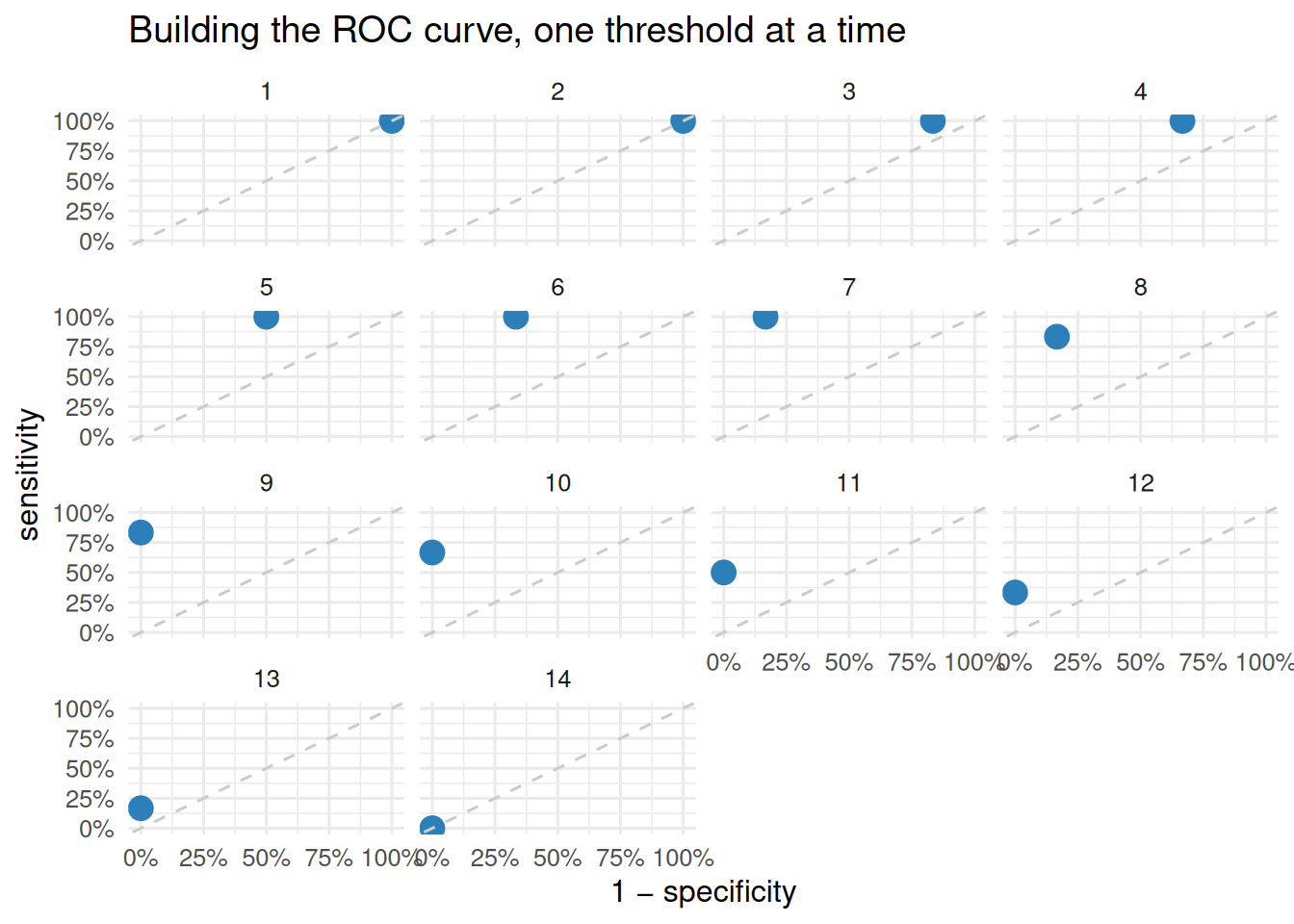
16.10.5 The receiver operating characteristic (ROC)
Instead of choosing one threshold, we can look at model discrimination across all possible thresholds.
iteration
threshold
plot
1
-Inf
2
0.1
3
0.25
4
0.35
5
0.44
6
0.49
7
0.57
8
0.61
9
0.68
10
0.7
11
0.78
12
0.82
13
0.95
14
Inf
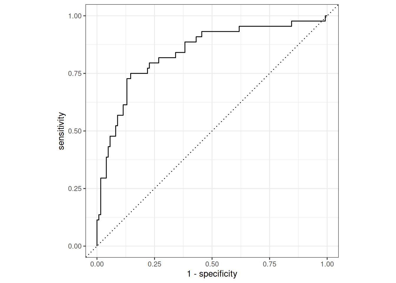
The ROC curve shows sensitivity against 1 − specificity.
AUC can be interpreted as the probability that the model assigns a higher predicted probability to a randomly chosen “impaired” observation than to a randomly chosen “control” observation.
AUC measures discrimination. It does not tell us whether the predicted probabilities themselves are accurate.
16.11 Calibration
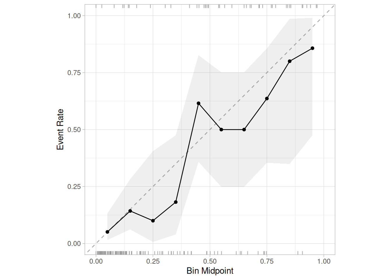
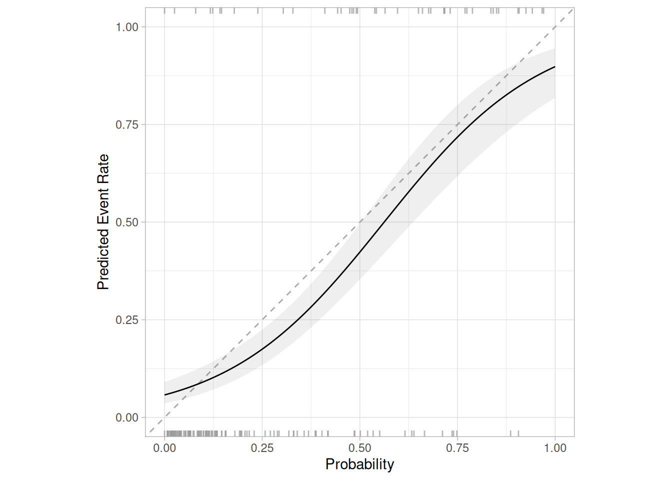
Calibration refers to the agreement between observed endpoints and predictions. For example, if we predict a 15% risk that a patient will have cognitive decline, the observed proportion should be 15 MCDs per 100 with such a prediction. As always, we recommend visualizing this in a plot with predictions on the x-axis and the observed endpoint on the y-axis, see Figure 16.2. The observed values on the y-axis are 0 or 1 (cognitive impairment/ control), while the predictions on the x-axis range between 0 and 100%.
Perfect predictions should be on the ideal line, described with an intercept alpha (‘A’) of 0 and slope beta (‘B’) of 1. The log odds of predictions are used as the predictor of the 0/1 outcome.
16.11.1 Alpha: calibration-in-the-large
The intercept A relates to calibration-in-the-large, which compares the mean of all predicted risks with the mean observed risk. The parameter hence indicates the extent that predictions are systematically too low or too high.
When assessing external validity, some countries might have higher prevalence, which will invalidate the model. This test is called geographical validation. Another type of validation, called temporal validation, use data from a different year (or century). It is often the case that prevalences change over the course of time and outdated data cannot generalize to the modern medical standards and practices.
16.11.2 Beta: calibration slope
The calibration slope B is often smaller than 1 if a model was developed in a relatively small data set. Such a finding reflects that predictions were too extreme: low prediction too low, and high predictions too high.
For the model based on 167 patients, the slope was 0.639 among the internal validation patients, in line with what was expected at internal validation (shrinkage factor 0.82). For the model based on MORE?, B was close to one at internal validation by cross-validation or bootstrapping, as well as at external validation in non-US patients (slope 0.99, p = 0.55 for comparison with slope = 1), see Figure 16.2.
In R, the calibration model can be written as a normal logistic regression using {glm}:
calibration_model<-ad_validation_logistic|>mutate( outcome =Class=="impaired", logit_p =log(.pred_impaired/(1-.pred_impaired)))|>glm(outcome~logit_p, data =_, family =binomial)broom::tidy(calibration_model)
Calibration is about the accuracy of the probabilities. A model can have excellent discrimination and poor calibration.
16.12 Discrimination using the concordance statistic
Discrimination refers to the ability of the model to distinguish a patient with the endpoint (cognitive impairment) from a patient without (control). A better discriminating model has more spread between the predictions than a poorly discriminating model.
Consider the extreme example where a model predicts all subjects to have the same predicted risk as the incidence. This model would have perfect calibration — but it would be useless since it does not discriminate between patients! 😅
A validation plot showing a wide spread between predictions as a histogram, or between deciles of predicted risk, indicates a good discriminating model, see Figure 16.2.
We use the concordance (c) statistic as an outcome for the models ability to discriminate between groups. For a binary endpoint, c is identical to the area under the receiver operating characteristic (ROC) curve, which plots the sensitivity (true-positive rate) against 1 – specificity (false-positive rate) for consecutive cut-offs for the predicted risk.
In our data, we have a AUC of 0.840
Intuition of C-statistic
Imagine you play a game with your model. You pick every possible pair of people from your data where one person had the event (1) and the other person did not (0).
You ask your model:
“Which of these two people had a higher predicted probability of the event?
There are three possible outcomes for each pair:
Concordant pair: The model assigns a higher predicted probability to the person who actually had the event (1) than to the person who did not (0).
Discordant pair: The model gets it backward and assigns a higher probability to the person who did not have the event (0).
Tied pair: The model assigns the exact same probability to both people.
The c-statistic is simply the percentage of pairs that are concordant (plus half of the tied pairs) out of all possible pairs.
While calibration and discrimination are important for validating prediction model, neither reflect real clinical usefulness. Clinical usefulness can be boiled down to the ability to make better decisions with a model than without.
If a prediction model aims to guide treatment decisions, a cut-off is required to classify patients as either low risk (no treatment) or high risk (treatment is indicated). The cut-off is a decision threshold.
You will learn about decision-curve analysis in Workshop 3.
D
The D component asks whether the predictions are useful for making decisions. That requires specifying a clinical action and the range of probability thresholds at which that action would be taken.
16.14 Internal and external validation
Everything we’ve done so far has been an internal validation — what do I mean by that?
Recall that we initially made an arbitrary split of the data: all odd-numbered patient IDs were assigned to a test set and the even-numbered IDs to a validation set. Had we used all the data for our model, we could not have performed any independent validation!
16.14.1 Internal validation
Validating internally — using data from the same study or dataset that was used to develop the model — is useful for several reasons.
First, it allows us to estimate how well our model is likely to perform on new patients from the same target population. We can use part of our data to develop the model and hold back another part to evaluate its performance.
However, simply making one arbitrary split into training and validation data has some disadvantages. The estimated performance can depend heavily on which patients happen to end up in each set. With a small dataset, this can lead to substantial uncertainty in our estimate of model performance.
Cross-validation is a more robust way of making internal splits.
In \(k\)-fold cross-validation, we divide the data into \(k\) roughly equal-sized groups, or folds. We then:
Fit the model using \(k - 1\) folds.
Evaluate the model on the remaining fold.
Repeat this process until every fold has been used as the validation data.
Average the results across all folds to obtain an estimate of model performance.
For example, in 5-fold cross-validation, each patient is used for validation once and for model development four times.
Cross-validation therefore makes more efficient use of a limited dataset than a single train/test split. It is particularly useful when the available dataset is relatively small.
Importantly, cross-validation is still internal validation. The patients used to evaluate the model come from the same underlying study and therefore may share characteristics with the patients used to develop the model.
16.14.2 External validation
Validating externally — using data from other studies, hospitals, populations, or settings — is necessary if we want to know whether a model generalises beyond the data on which it was developed.
A model can perform very well during internal validation but perform much worse when applied to new data. This can happen because the new patients, clinical practices, measurements, or disease prevalence differ from those in the development dataset.
External validation therefore provides a much stronger test of whether a prediction model is likely to be useful in practice.
There are several ways in which we can perform external validation.
Temporal validation:
Develop the model using data from an earlier time period and evaluate it using patients from a later time period. This tests whether the model continues to work as patients and clinical practice change over time.
Geographical validation:
Develop the model using data from one geographical location, such as a hospital or country, and evaluate it using data from another location. This tests whether the model generalises to a different population or healthcare setting.
Domain validation:
Develop the model in one type of healthcare setting and evaluate it in another. For example, a model developed using patients from a specialist hospital could be evaluated in primary care.
Cross-setting validation:
Develop the model using one study and evaluate it using an entirely independent study. This is often the strongest form of external validation because the validation data were collected independently of the model development process.
The further the external validation data are from the development data, the more demanding the test of generalisability becomes.
16.14.3 When to use internal and external validation?
Internal and external validation can be seen as two levels of evidence:
Internal validation as the initial an inexpensive validation:
Statistical estimation of overfitting/underfitting
Best guess for future external validation and generalizability
Always possible
External validation as the necessary validation check:
Does my model still perform well when applied to genuinely new data from > another time, place, setting, or study?
A model should therefore not be considered ready for widespread clinical use simply because it performs well on its development data or under internal validation. External validation is needed to establish whether the model generalises to the population and setting in which we ultimately want to use it.
16.15 Effect size estimation
Prediction performance and effect estimation are different questions.
A logistic regression coefficient describes the association between a predictor and the outcome. For example:
How much does the odds of “impaired” change for a one-unit increase in age?
The dataset used here contains only the predictions, not the original predictors. Therefore, we cannot recover the original regression coefficients or their odds ratios from ad_validation_logistic.
What we can estimate is the association between the model’s predicted risk and the observed outcome. The calibration slope above is one such measure.
This distinction is important:
Prediction asks: How accurately can we predict what will happen?
Effect estimation asks: How does changing a particular variable relate to what happens?
A model can be excellent for prediction without giving an unbiased estimate of a causal effect.
16.15.1 Effect size calculation in R:
Binary and survival outcomes have three criteria:
Small overfitting: expected shrinkage of predictor effects ≤ 10%
Small absolute difference (≤ 0.05) between apparent and adjusted Nagelkerke’s R²
Precise estimation (within ± 0.05) of the average outcome risk at the timepoint of interest
Calculate the minimum sample size for a logistic prediction model with 24 candidate predictor parameters, an anticipated outcome prevalence of 17.4%, and a Cox-Snell \(R^2\) of 0.288 (taken from an existing model):